QSAR: Principles and Methods
Info
Quantitative Structure Activity Relationship (QSAR) is involved in building mathematical models for correlating molecular structures with molecular properties. In this section we introduce the notion of molecular descriptors and present the QSAR model and its validation.
Number of Pages: 113 (±2 hours read)
Last Modified: May 2008
Prerequisites: None
Introduction to QSAR
Molecular Structure and Molecular Properties
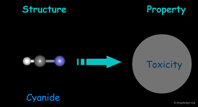
One of the most pervasive postulates in the life sciences is that all molecular properties are coded by and consequently result from molecular structure. Some examples of structure-property relationships are illustrated on the following pages.

Structure-Property Relationships: Example 1
Paracetamol selectively inhibits the cyclooxygenase enzyme COX-3 found in the brain and spinal cord and consequently relieves pain and reduces fever.

Structure-Property Relationships: Example 2
Cyanide exerts its toxicity by inhibiting cytochrome-c oxidase, the terminal enzyme of the respiratory chain, leading to insufficient utilization of oxygen and suffocation. Inhibition occurs through binding to the ferric ion of the cytochrome.
Structure-Property Relationships: Example 3
Saccharin (usually sold as sodium saccharin) binds to the sweet taste T1R3 receptor located in the plasma membrane of the sweet-taste sensory cells located in the taste buds. Binding of saccharin to T1R3 initiates a cascade of events in the taste-sensory cell that eventually releases a signaling molecule to an adjoining sensory neuron, causing the neuron to send impulses to the brain. In the brain, these signals cause the actual sensation of sweetness.

What is QSAR?
Molecules exert their biological effect by binding to their respective receptors, a phenomenon that in turn is governed by their molecular structures (and the molecular structure of the receptor). QSAR (Quantitative Structure Activity Relationship) attempts to formulate the relationship between structure and activity as a mathematical model.

What is QSPR?
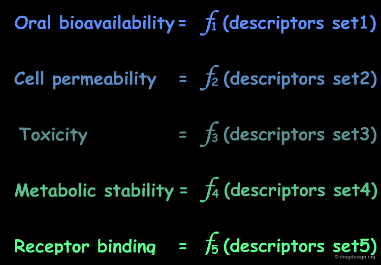
The biological effect is just one example of molecular properties. QSPR (Quantitative Structure Property Relationship) is an extension of QSAR and is designed to formulate the relationship between structure and any molecular property as a mathematical model. Other properties include for example: solubility, oral bioavailability, metabolic stability and cell permeability.

Focus on a Single Property at a Time
No single QSPR model can capture the direct connection between all the properties of a compound and its molecular structure; only a single property is handled at a time.
Molecular Descriptors
Thus, the derivation of a direct relation with the molecular structure of one single property is extremely challenging. However, structural factors known as molecular descriptors that influence the molecular property can be identified. For this reason, the QSAR model correlates the property with molecular descriptors.

Examples of Molecular Descriptors
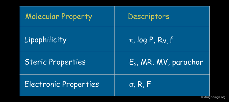
Examples of molecular properties with their associated descriptors are listed in the following table. Later on in this chapter the nature and the meaning of some QSAR descriptors are presented.
The QSAR Equations
All QSAR equations have a molecular property expressed as a function of specific descriptors. They differ in terms of the property they are attempting to correlate, the descriptors they use and the mathematical expression of the model.
Types of Molecular Descriptors
Molecular descriptors can be classified according to the dimensionality of the molecular structure from which they are derived. 1D descriptors are derived from the chemical formula, 2D descriptors are derived from a 2D (chemdraw-like) structure and 3D descriptors are derived from the 3-dimensional structure.

Molecular Descriptors: 1D
The chemical formula constitutes a 1-Dimensional representation of the molecular structure from which 1D descriptors can be derived. Such descriptors are based exclusively on the type of atoms which make up the molecule.

Molecular Descriptors: 2D
A Chemdraw-like structure constitutes a 2-Dimensional representation of the molecular structure from which 2D descriptors can be calculated. In addition to types of atoms, 2D descriptors also incorporate the bonding pattern of the molecule.

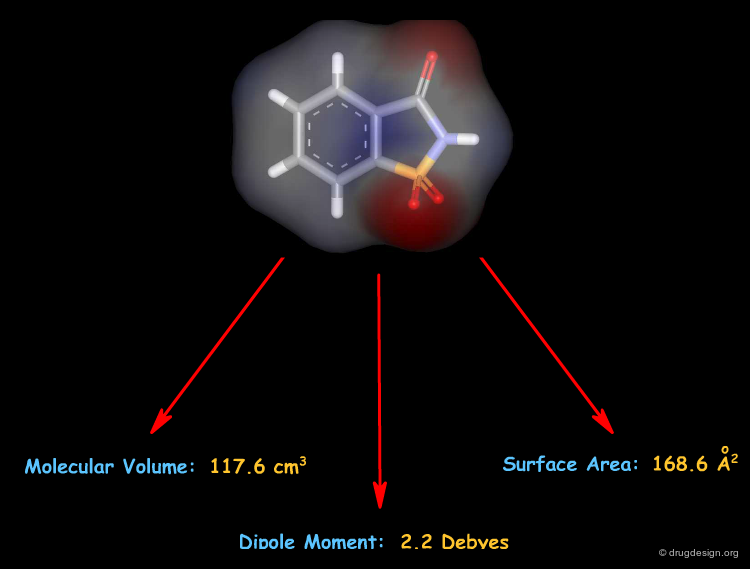
Molecular Descriptors: 3D
3D descriptors derived from a 3D molecular structure take the spatial arrangement of the atoms in the molecule into account.
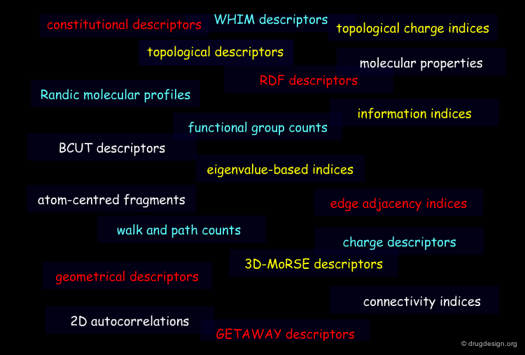
A Multitude of Molecular Descriptors
The number of descriptors that can be derived from a molecular structure is virtually unlimited. Currently available software packages can calculate thousands of descriptors. For example the DRAGON program calculates 1612 descriptors distributed into 20 categories.
book
Todeschini R and Consonni V the Series of Methods and Principles in Medicinal Chemistry - Volume 11 WILEY - VCH 2000
Biologically Relevant Descriptors
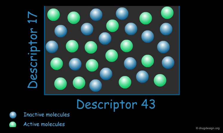
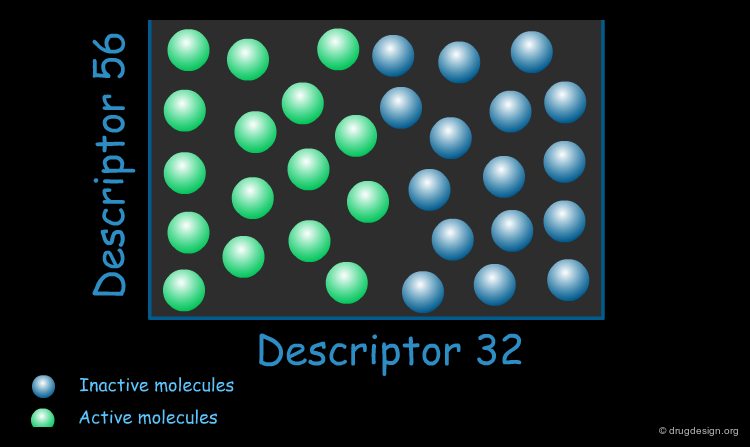
When constructing a QSAR model, the key is to use descriptors that are relevant to the specific property of interest. These "biologically relevant descriptors" help generate a model that differentiates between molecules that possess the property of interest and those that do not.

Application of QSAR
QSAR models are built for three main reasons: to understand the relationship between structure and activity, design compounds with improved activity, and predict the activities of compounds prior to their synthesis. These reasons in fact adhere to the rational sequence of a QSAR analysis project where the first step is to understand the phenomenon, and then use this understanding to design new compounds.

Understanding Structure-Activity Relationships
A good model can reveal information about the receptor's binding site. For example a correlation with electronic descriptors may indicate that the biological activities could be due to the chemical reactivity of the compounds, or alternatively, a correlation with hydrophobic descriptors may reveal the existence of a hydrophobic pocket in the receptor.

Designing Compounds with Improved Activities
Once a QSAR model is obtained and reproduces the known data satisfactorily, it can be exploited to predict the biological activity of not yet synthesized analogs. This is of paramount importance in lead optimization and represents one of the most popular uses of the QSAR approach.

Reducing a Virtual Library to a Practical Size
The recent explosion in combinatorial chemistry has added a new dimension to the QSAR approach by reducing a huge virtual library to a manageable size for combinatorial synthesis and high through-put screening.

The Foundations of QSAR
Birth of QSAR
QSAR dates back to the 19th century with the work of Cros (1863) who first observed an inverse correlation between the toxicity of alcohols and their water solubility. Other important milestones include work by Crum-Brown and Frazer who related physiological action to chemical constitution (1868). A few years later Horst, Overton and Richet independently observed that the toxicity of organic compounds depended on their lipophilicity/solubility. This discovery was followed by research by Meyer and Overton, who proved that anesthetic potency correlated well with partition coefficients (1899).

The Foundations of QSAR
During the first half of the 20th century, Louis Hammett laid the foundation for modern QSAR by correlating electronic properties of organic acids and bases with their equilibrium constants and reactivity. An important landmark in the development of QSAR took place in 1964 with the introduction of the Free-Wilson method and Hansch analysis. This section covers these three seminal contributions to QSAR in some detail.

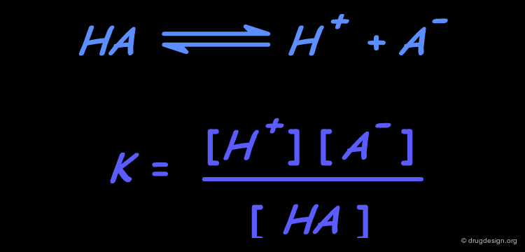
The Hammett Contribution
The dissociation of HA organic acids is a process by which a proton (H+) is removed from the neutral compound, leaving behind a negatively charged species (A-). The extent of the reaction is measured by the dissociation constant K. Louis Hammett observed that the dissociation constants of aromatic acids are influenced by the electronic properties of the substituents on the phenyl ring.
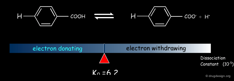
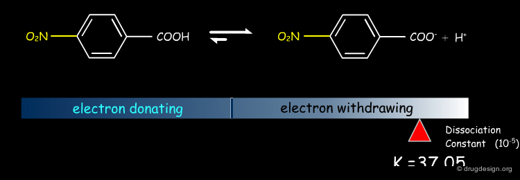
Dissociation Constants of Substituted Benzoic Acids
The dissociation constants of substituted benzoic acids indicate that electron withdrawing groups increase dissociation while electron donating groups decrease it.


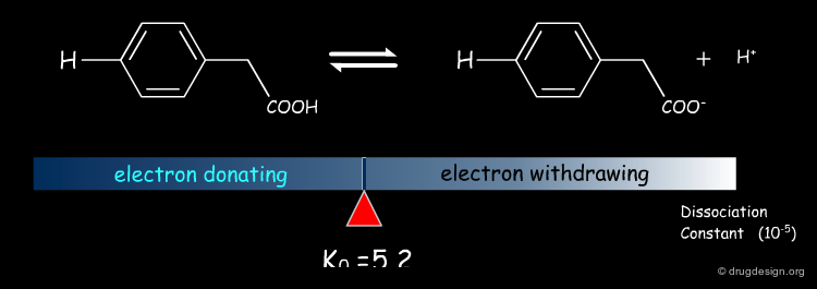
Dissociation of Substituted Phenylacetic Acids
A similar effect exists for other equilibria such as substituted phenylacetic acids.


Linear Free Energy Relationship
When plotting the quantity log(K/Ko) for benzoic acids on the X axis, where K and Ko refer to the substituted and unsubstituted compounds, respectively, and the corresponding values measured for the same set of substituents in phenylacetic acids on the Y axis, Hammett obtained a straight line. Because of the association between dissociation constants and free energies [ΔG=-RT Log(K)] this phenomenon is known as the linear free energy relationship.

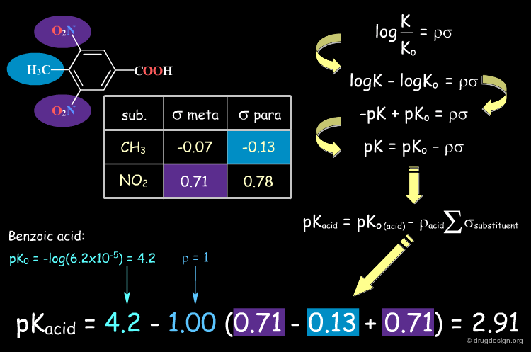
The Hammett Equation
The straight line described on the previous page can be written as a linear equation, the Hammett equation. Note that Ρ is related to a given scaffold (e.g. phenylacetic acids), whereas a Σ is a descriptor of a substituent and describes its influence on the dissociation constant. It is positive for electron withdrawing substituents and negative for electron donating substituents.

wikipedia
The Meaning of Ρ
Ρ describes the magnitude of the effect a substituent can exert on the dissociation reaction of a given scaffold. As the distance between the substituent and the dissociated proton increases, its influence on the dissociation reaction decreases and so does the value of Ρ.


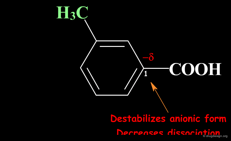
The Meaning of Σ
Σ describes the effect of substituents on the dissociation reaction. Substituents on the phenyl ring can increase or decrease the equilibrium constant by stabilizing or destabilizing the anionic form via the formation of a positive or negative partial charge at C1.
Examples of Σ Constants
Electron donating substituents have negative Σ values, whereas positive Σs correspond to electron withdrawing groups. Note that Σ values differ depending on whether the substituent is meta or para (sigma values are clickable).

Predicting the pKa of Benzoic Acid Compounds
The Hammett equation is an example of a QSPR equation. It correlates a molecular property, the dissociation constant, with a set of molecular descriptors (Σ and Ρ). It can be used to predict the pKa of benzoic acid analogs. When a molecule has multiple substituents, the Σ values are summed to yield the total value for the compound, as shown in the following example.
Hansch Contribution
Corwin Hansch recognized the importance of lipophilicity for biological activity. Lipophilicity can be defined as the tendency of a compound to prefer an organic phase rather than an aqueous phase. Molecular lipophilicity is correlated with the presence of hydrophobic groups (e.g. aromatic rings) and with the absence of polar and ionizable groups.

The Importance of Lipophilicity
To exert its biological effect, a drug must reach its site of action. On its way, the compound encounters biological barriers. For example, the cell membrane is composed of a lipid bilayer, therefore lipophilic compounds are able to penetrate such barriers. The lipophilicity thus determines in part the amount of the compound that reaches the target site.

LogP is a Measure of Compounds Lipophilicity
LogP describes the lipophilicity of a compound, and is the measure of the partitioning of this compound between a lipidic phase (usually 1-octanol) and an aqueous phase. It is represented by a partition coefficient P or by its log value. Compounds with P>1 (logP>0) are lipophilic whereas compounds with P<1 (logP<0) are hydrophilic.

Correlation of LogP with Biological Activities
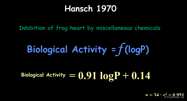
Hansch observed that in several compound series, the biological activities (inhibition of frog heart) correlated well with logP. The resulting QSAR expression turned out to be quite simple: a linear equation.
Example of Correlation with LogP
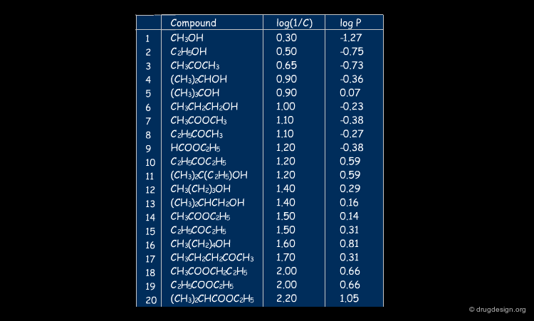
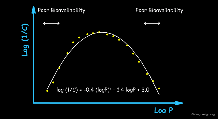
A correlation with logP was found for the isonarcotic activities of diverse esters, alcohols, ketones, and ethers (structures, biological activities and logP are shown by clicking the button "training set"). The training set covers a large range of values for logP and the model generated is quite simple. In the equation log(1/C) represents the biological activity response.

articles
QSAR studies on drugs acting at the central nervous system S. P. Gupta Chem. Rev. 89 1989
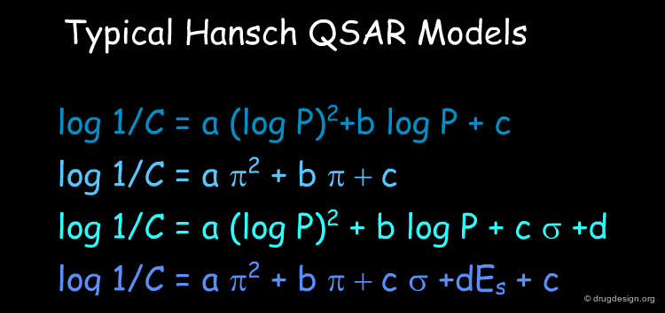
Improvements of the Initial Model
When attempting to ameliorate his initial idea (only one descriptor), Hansch further refined the QSAR equation and introduced other descriptors such as Σ (electronic), Es (Taft), π (lipophilicity), MR (Molar refraction) that represent properties that may influence drug action. He also considered other mathematical equations likely to represent the behavior of the biological system. The analytical forms of some of the typical QSAR models he developed are indicated below, whereas the most common descriptors used in Hansch's analyses are presented in the following pages.
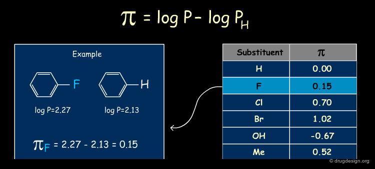
The π Descriptor
The π descriptor characterizes the lipophilicity of a substituent. It is defined as the difference between the logP of the substituted and unsubstituted compounds. Substituents that are more hydrophobic than H have π positive values, whereas substituents less hydrophobic than H have negative values. The π values for several common substituents are listed below, and an example is provided.
The MR Descriptor
Molar refractivity (MR) is a molecular descriptor that contains information on the compound's volume corrected by the refractive index (the ratio of the velocity of light in a vacuum to the velocity of light in the substance of interest). In the definition below, d is the density and n is the refractive index. Several MR values are listed below.

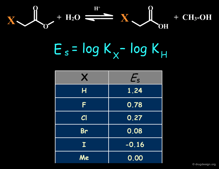
The Taft Descriptor (ES)
The Taft steric constant Es is an experimental value based on rate constants for a given model reaction. It is a measure of the steric effect exerted by a substituent on the equilibrium. In the definition below Kx and KH are the rate constants for substituted and unsubstituted compounds. The bulkier the substituent, the more negative the Es. The table lists Es values for several common substituents.
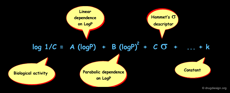
Meaning of Parabolic Dependence on LogP
Hansch's introduction of a parabolic term for logP was a breakthrough that helped make QSAR a more powerful tool. This additional term denotes the existence of an optimum in logP: molecules with higher values start to be trapped in hydrophobic membranes and cannot reach their site of action.

The Free-Wilson Analysis
In 1964, Free and Wilson derived a mathematical model based on the hypothesis that overall biological activity is the sum of all elementary contributions of the substituents. This approach assumes that substituent effects are additive.

articles
A Mathematical Contribution to Structure-Activity Studies Free, S. M., Jr.; Wilson, J. W. J. Med. Chem. 7 1964
Indicator Variables and Substituent Weights
In the Free-Wilson model biological activity is represented by the following equation. Indicator Variables xi (with values of 1 or 0) describe the presence or the absence of certain substituents at each scaffold position. The weight of each substituent is represented by the ai coefficients. µ is the overall average activity.

Free-Wilson Structural Matrix
The construction of the Free-Wilson QSAR model is based on a structural matrix composed of the xi indicator variables.

Example of Structural Matrix
An example of a matrix for a set of 22 disubstituted N,N-dimethyl-α-bromophenethylamines with antiadrenergic activities is given below.
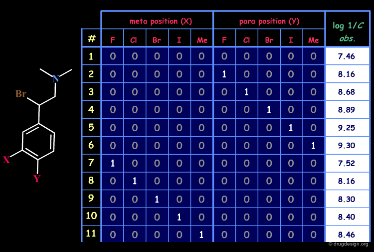


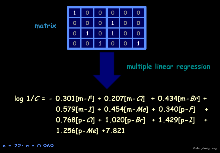
Example of Free-Wilson Equation
A mathematical procedure known as multiple linear regression is used to derive the QSAR equation from the structural matrix, ultimately leading to the values of ai and µ for the 22 antiadrenergic agents.
Predictability of the Model
The experimental and calculated values of the antiadrenergic molecules of the training set are indicated below and show that the Free-Wilson model reproduces the biological activities well. Moreover the equation can be used to predict the biological activities of new not yet synthesized analogs.

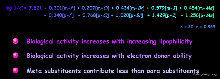
Understanding the Molecular Determinants
By examining the QSAR equation, we can draw several conclusions regarding the influence of the various substituents on activity. For example meta substituents contribute less than the para; the biological activity increases with electron donor ability etc...
Design of a QSAR Model
Embarking on the Design of a QSAR Model
The planning of a QSAR model must be carefully managed. In this section we will explore the methodology for designing a QSAR model in some detail, present the ideas and statistical concepts behind the QSAR model, the rules that need to be followed and the errors that should be avoided.

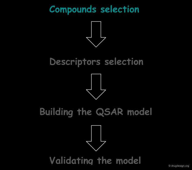
The Four Steps
To construct a QSAR model the following steps should be followed: (1) assemble a sufficiently large and diverse set of compounds along with their biological activities; (2) select a set of descriptors which is likely to be related to the biological activity of interest; (3) formulate a mathematical equation that reflects the relationship between the biological activity and the chosen descriptors, and finally (4) validate the QSAR model.

An Iterative Process
Constructing a QSAR model is an iterative process. First, the QSAR equation is derived from an initial set of descriptors. Attempts are then made to improve this model by adding or removing descriptors and refining the mathematical equation, in an iterative fashion.

Compounds Selection: Step 1
Compounds Selection
The selection of the compounds is the first step in building a QSAR model and consists of assembling a sufficiently large and diverse set of compounds with known biological activities. The molecules should be selected with great care in order to define a set of compounds that is homogenous and represents the system well.
Predictions by Interpolation
The compounds selected for a QSAR analysis should cover a large range of values for those descriptors believed to be relevant to biological activity. This increases the probability that future compounds will have descriptors within this range and allow predictions to be interpolative rather than extrapolative. As a rule, interpolative predictions are more accurate than extrapolative predictions.

Example of Extrapolative Model
Extrapolating a model for values that are outside the range of the training set may lead to incorrect predictions. In the following example the experimental points lie in a straight line, however at higher values the model is more complex and no longer linear.

Identification of Outliers
QSAR modeling is based on the assumption of homogeneity and an absence of influential outliers in the training set. An outlier can be a molecule acting according to a different mechanism of action, an improper biological activity as reported by another laboratory, or simply an incorrect value (experimental or typographic error). Repeat measurements of biological activities and using the greatest number of molecules helps reduce the distortions introduced by outliers.


articles
Outliers in SAR and QSAR: Is unusual binding mode a possible source of outliers?
Ki Hwan Kim
J Comput Aided Mol Des.
21(1-3) 2007 10.1007/s10822-007-9106-2
Biological Activities in Terms of Log 1/C
To reflect the free energy variations that occur in the biological action, biological activities are expressed as the logarithm of the concentration of the compound (log[C] or log 1/[C]), where C is the concentration of the compound required to produce a given standard response. In the following set of equations E and S represent respectively, the enzyme and the substrate. Biological activities should be accurate and span at least 2-3 orders of magnitude.

Descriptors Selection: Step 2
Descriptors Selection
As mentioned earlier in this chapter, the number of available descriptors for QSAR analyses is very large. A good model is based on a small number of well-chosen descriptors. When many descriptors are screened, a fortuitous correlation may occur. In the following pages important rules for the selection of relevant descriptors are presented.

Methods for Selecting Relevant Descriptors
Relevant descriptors can be selected either manually or by using automated approaches. For each method, computer programs are available that help in the selection of relevant descriptors.

Manual Selection of Descriptors
The manual method is based on a thorough understanding of the SAR and exploiting intuitions generated by the analyses. For example if preliminary analyses indicate that steric or hydrophobic substituents may increase activity, descriptors such as the molar refractivity (MR) and the hydrophobic substituent constant, π should be selected in the first place.

Automated Selection of Descriptors
The second method looks at the selection of descriptors in an automated manner, using programs that score and rank them. Automated and manual methods can also be combined to select relevant descriptors and select those that are easy to interpret. Modern methods use genetic algorithms based on natural evolution principles (Darwin).

Systematic Combination of Descriptors
In principle the identification of the best descriptors can be accomplished by a systematic evaluation of all their combinations. For each combination, a QSAR equation can be derived and then ranked. The highest-ranked equation will reveal the best subset of descriptors. However this systematic approach is not always feasible: for n descriptors (current software can process 2000), there are 2n-1 different combinations (subsets). In the following pages we present automated methods that circumvent this difficulty.


Methods for Selecting a Subset of Descriptor
"Forward regression", "backward elimination" and "stepwise regression" are methods for selecting a subset of descriptors from a large descriptor pool. The process starts with an initial subset of descriptors, then successive small alterations of this subset are made and assessed. If this modification improves the model, the change is accepted, otherwise it is rejected. The treatment is terminated when it is not possible to improve the model further.

Forward Selection
The "forward selection" method starts with the single descriptor which best correlates with the dependent parameter. At each subsequent step the method adds the next most contributing descriptor. The process stops when the addition of a descriptor does not improve the model's performance as assessed by appropriate statistical indices.

Backward Elimination
The "backward elimination" method starts with a model that includes all the descriptors. At each step the method removes those descriptors that do not degrade the model's performance. The process is stopped when performance starts to decline as assessed by relevant statistical indices.

Stepwise Regression
The "stepwise regression" method starts (like in forward selection) with the single descriptor that best correlates with the dependent parameter. At each subsequent step the method adds the next most contributing descriptor and can potentially remove non-contributing descriptors. The process is stopped when additional descriptors do not improve the model or when removing descriptors causes the model's performance to decline, as assessed by appropriate statistical indices.

Scaling Descriptors
Descriptors represent a broad range of physico-chemical properties. They need to be calibrated in order to provide a good balance of their respective influence when they are combined. Scaling treatment consists of a mathematical operation called "normalization" which sets boundaries for the variation of each descriptor.

Correlation Between Descriptors
When two descriptors essentially convey the same information about a series of molecules they are said to be correlated. The use of correlated descriptors in the same equation must be avoided, because the information they characterize is over-represented when both are present. A "correlation matrix" provides useful information on the degree of correlation of different pairs of descriptors.

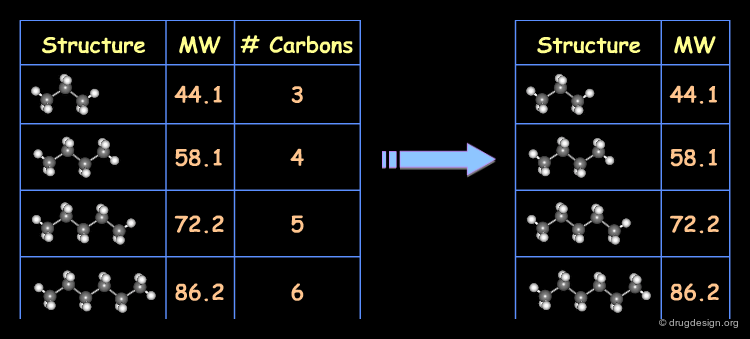
Example of Correlated Descriptors
Consider for example the molecular weight and the number of carbon atoms as two descriptors characterizing a series of alkanes. These two descriptors are highly correlated, which can be shown graphically.

Solution to the Problem of Correlated Descriptors
When two descriptors are highly correlated, the solution is to remove one of them. The descriptor that carries strong structural information is preferred and the less intuitive one is removed. An alternative solution consists of removing the descriptor that has the highest correlation with the other descriptors.
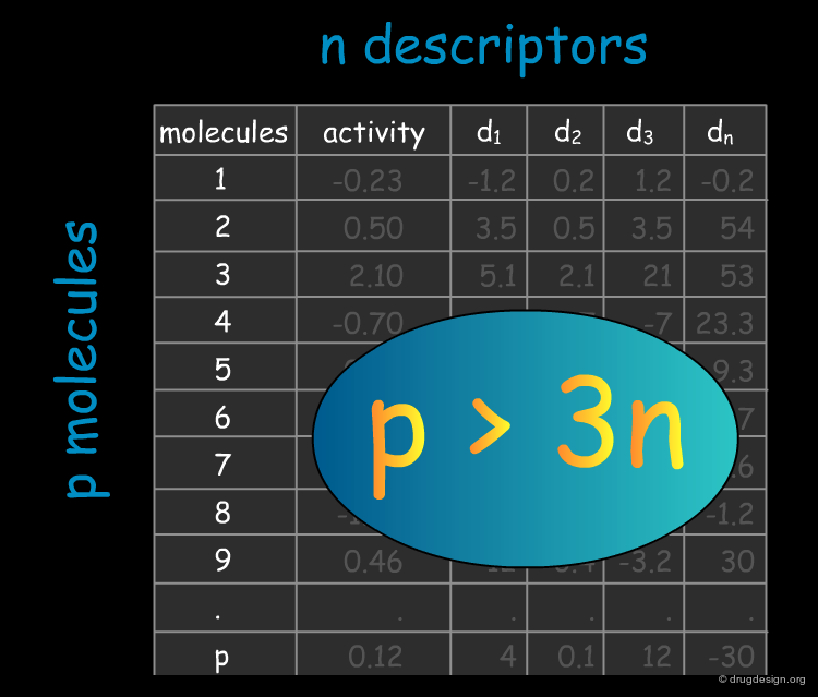
The Holy Grail in QSAR
There is a general consensus that in a meaningful QSAR equation, the number of molecules in the training set should exceed the number of descriptors by a factor of 3 to 5.
articles
Chance Factors in Studies of Quantitative Structure-Activity Relationships Topliss, J. G.; Edwards, R. P. J. Med. Chem. 22 1979
Deriving the Equation: Step 3
Deriving The QSAR Equation
Step 3 consists of deriving the QSAR equation corresponding to the set of descriptors that were selected in the previous step.

The Starting Point: The Study Table
The starting point for deriving a QSAR equation is the study table. It consists of a spreadsheet with molecules across the rows and molecular characteristics (biological activity, descriptors) down the columns. Typically, the first column indicates the molecular identification (e.g. compound number or name, 2D structure), the second column its activity, and subsequent columns the values of the corresponding descriptors.

Graphical Analysis of the Data
The study table should lead to graphical analyses. This step is of paramount importance and leaves room for "hunches" and preliminary interpretations. This is where the key questions are asked: is there an order? Are the points distributed according to known patterns? Can the recognized trends be translated into physico-chemical expressions? etc...

Choice of the Mathematical Equation
After having identified trends in the system, the correlation process can begin. The initial analyses help guide the choice of the right mathematical equation. This equation should not be treated as a black-box; rather it should contain information that reflects the behavior and allows for interpretation of the system in a structural manner. Sound structural informational content in a QSAR equation is of utmost importance for formulating step 3.

Complexity Levels and Data Overfitting
The next hurdle is the mathematical equation. At this stage the complexity of the model depends on both the form of the mathematical equation and the number of descriptors considered.

Mathematics are Very (too) Powerful
QSAR models can be skewed unintentionally by overly powerful mathematical choices. An equation that fits the data of a training set precisely can yield an equation that is perfect mathematically but meaningless for molecules other than those in the training set. For example if the training set consists of 20 molecules, it is always possible to select a set of 20 randomly chosen descriptors and solve the mathematical system for 20 equations and 20 unknowns. This error is known as data-overfitting.
Illustration with an Example
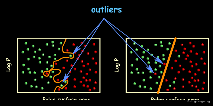
To illustrate the data-overfitting problem, let's take a series of compounds for which the permeability through the blood brain barrier (BBB) has been found to be correlated with their logP and polar surface area. In the following graph we have plotted a hypothetical series of compounds in this space and color-coded them according to their BBB permeability. Compounds colored green are permeable whereas compounds colored red are not.
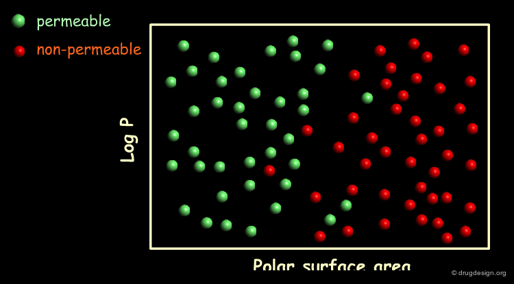
A Simple Model
A linear model for differentiating between BBB permeable and BBB impermeable compounds can be formulated by drawing a straight line through the logP / Polar surface area space. Most of the compounds on the left side of the line are BBB permeable whereas most of the compounds on its right are BBB impermeable. As the model correctly classifies 45 out of the 50 compounds it has a success rate of 90%.

A Complex Model
A model with an improved success rate can be generated by drawing a curved line across the logP / Polar surface area space. This model completely separates the BBB permeable compounds from the BBB impermeable compounds and thus has a success rate of 100%.

Comparing the Two Models
Which of the two models better distinguishes BBB permeable from BBB impermeable compounds? Clearly the complex model has a higher success rate. However, by doing so it distorts its shape to correctly classify the outliers thereby completely reflecting the scatter of the training data - it is therefore an overfitted model. On the other hand, the simple model mislabels the outliers on the assumption that they are indeed outliers.
Predictive Power of the Simple Model
The simple model predicts that all test compounds lying to the left of the line are BBB permeable and all those lying to the right of the line are BBB impermeable. Assuming that the test compounds are similar to the training compound, the prediction power of this model is expected to be high.

Predictive Power of the Complex Model
The complex model also predicts that all test compounds lying to the left of the line are BBB permeable and all those lying to the right of the line are BBB impermeable. However, under the same assumption of similarity between test compound and training compound, many of its predictions are expected to be erroneous.

Complexity Dictated by Predictability of the Model
In the QSAR approach tailoring an equation to the peculiarities of a training set is not a problem. However, forcing the mathematics to fit too closely to the data may lead to meaningless models in terms of predictability (tools for assessing the predictability of a QSAR model will be presented in Step 4). The real issue is to stop the refinements early enough so that the predictive capabilities of the model are not lost.

Single Linear Equation: Mathematical Outline
The simplest form of a QSAR equation is a linear model with one descriptor. This simply yields the equation of a straight line of the form y = b0 +b1X where b0 indicates the intercept of the line with the y axis and b1 the slope of the line. b0 and b1 are calculated as described on the next page.

Calculating b0 and b1
b0 and b1 are calculated using the two equations indicated below. The details of such calculations are presented for the Capsaicin example under the heading "Example of simple linear regression".

Multiple Linear Regression: Mathematical Outline
It is not always possible to correlate biological activities with a single descriptor (linear model with one descriptor). Given that biological action results from the combined influence of many factors, one can extend the QSAR model to multiple descriptors. Indeed, the observation that several parameters used simultaneously can lead to good models prompted the development of a method referred to as "multiple linear regression" (MLR). In this model linearity is maintained for each of the individual descriptors.

Example: MLR vs. Single Linear Models
The example of anticonvulsant compounds shown below demonstrates that each descriptor Es, Σ and logP alone was not able to give a good correlation (r less than 0.40) with the biological activities. However, by using simultaneously logP and Σ, a significant improvement was made (r=0.80). The addition of Es improves the model even more (r=0.95). This indicates that the biological properties result from the combined action of lipophilicity, steric and electronic effects.

articles
PhD. Thesis C. Euvrard
Paris 1982
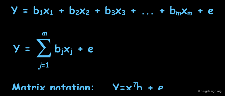
The Mathematics of MLR: a Single Sample
In MLR we try to express activity as a linear combination of descriptors. We recognize the fact that in most cases, our fit to the experimental data will not be perfect and error is usually unavoidable. In the equations listed below, y (the activity) is a scalar; xj is the value of the descriptor j and bj its associated coefficient; e is the error. In the matrix notation, xT is a row vector of the descriptors and b, a column vector of their associated coefficients.
The Mathematics of MLR: Many Molecules
For the case of multiple compounds, the activity values are assembled into a vector y of length n, where n is the number of compounds. The descriptors are collected into an n by m matrix where n again is the number of compounds and m is the number of descriptors. The coefficients are collected into a vector of length m and the errors are collected into another vector of length n.

The Solution of MLR
In the MLR formalism we search for the (unknown) set of coefficients b, which, when multiplied by the (known) descriptors, best approximates the (known) activity data (equation 1). A solution to this problem can be obtained through a matrix inversion procedure (equation 2).

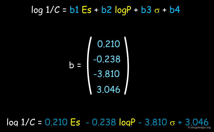
Analysis of the MLR Equation
One of the purposes of QSAR analyses is to understand the forces governing the activity of a particular class of compounds and to assist drug design. In the example shown below QSAR analyses reveal that the relative importance of the descriptors vary in the following order: logP > Σ > Es > MR; therefore the biological activities are governed in the first place by hydrophobicity (logP) and polarity (Σ) and to a lesser extent by steric effects (Es and MR).

Non-Linear Equations
A non-linear equation is an extension of a multiple linear regression. In some systems the linearity may not be sufficient to achieve a good correlation. Hansch was the first to introduce a parabolic term, and a complex biological process can be satisfactorily modeled by non-linear equations.

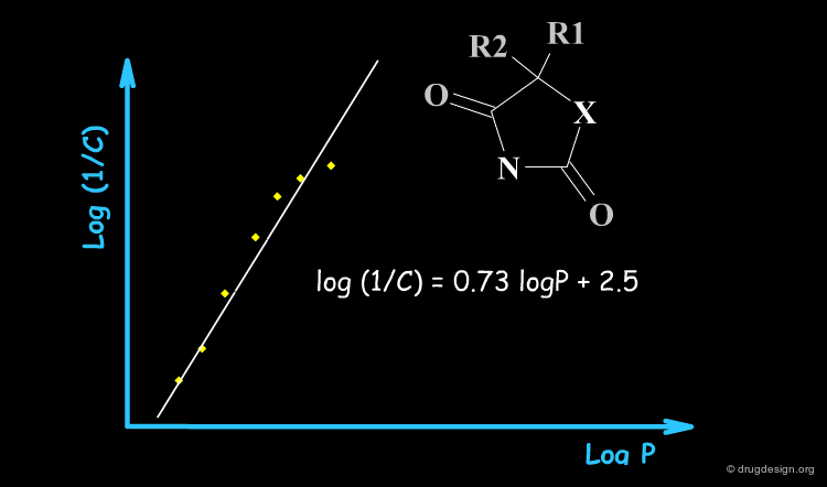
Example of Non-Linear Model
In the example below, the anticonvulsant activities of a set of molecules was initially found to be linearly correlated with logP. However, it is implausible to assume that the biological activity can increase indefinitely by increasing the lipophilicity of the molecules. It is known that highly lipophilic compounds cannot reach their site of action, because they are trapped in lipophilic environments. It is therefore more realistic to improve the initial model using a non-linear equation. The modified equation proved to be correct and revealed the existence of an optimum logP value, information that could not be derived from molecules with a small range of logP values.

Typical Non-Linear Equations
There are many reasons why the use of non-linear models is justified, including the kinetics of the drug transport, the equilibrium control of its distribution, allosteric effects, different pharmacokinetics, metabolism, solubility etc... The following are examples of non-linear models that have proved to be valid at least for special and complex biological systems.

Validating the Model: Step 4
Tools for Assessing the Quality of a Model
Efficient tools are necessary for assessing the validity of a QSAR model. Numerical analyses or statistical methods provide a variety of indexes that serve to evaluate the quality of the model and its limitations. In the following pages we present some of these tools and explain how to use them.

Predictive and non-Predictive Models
Broadly speaking there are two groups of indices: (1) those that indicate how well the QSAR equation can "reproduce" the experimental data and (2) those that can tell how far the model can be extrapolated to new molecules.

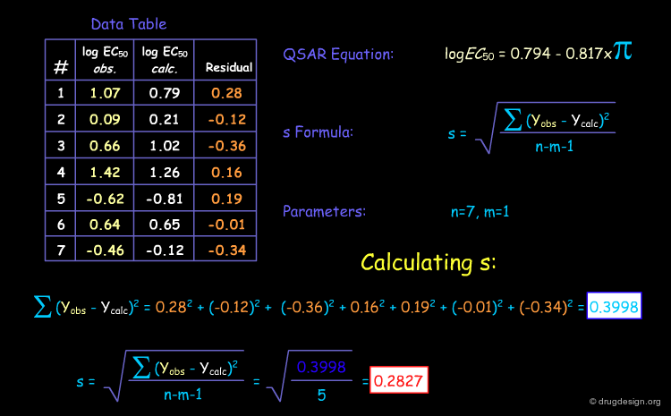
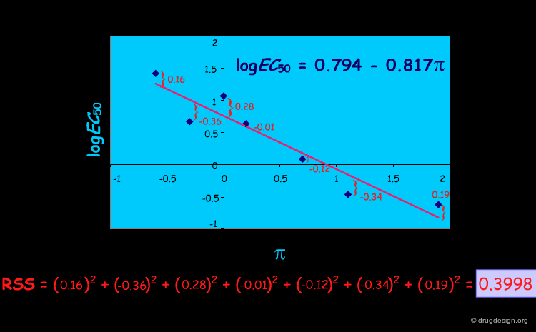
The Standard Deviation
The easiest way to "validate" a QSAR model is to calculate the standard error or standard deviation (SD or s), which is calculated as the average squared deviation of each number (the "residuals") from the mean. This index reflects how much the deviation between the data and the model is. The smaller the SD, the more the model is considered of good quality.

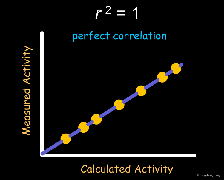
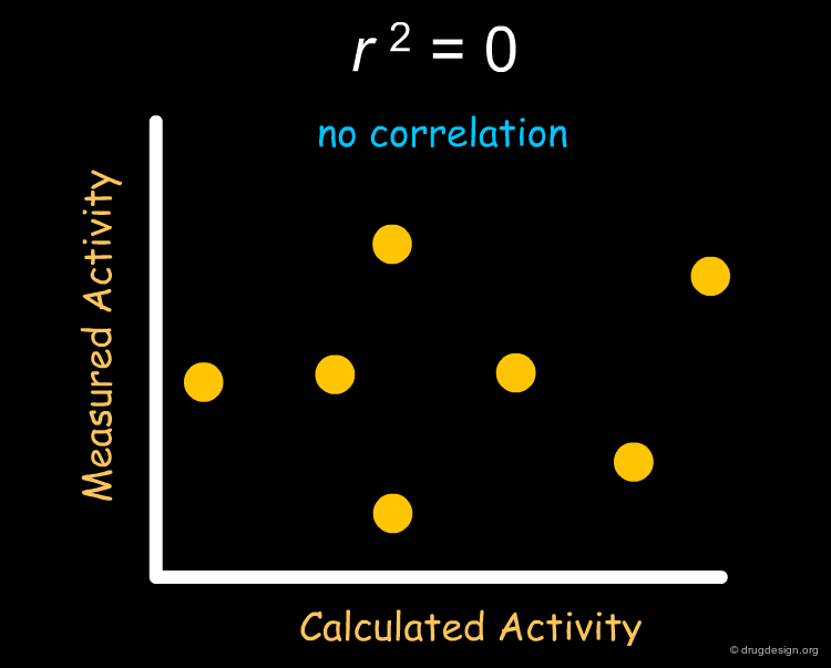
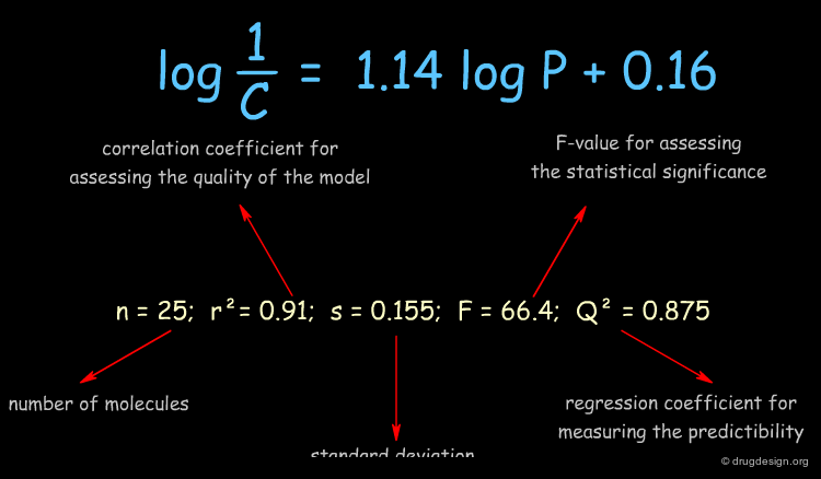
Correlation Index r2
The most frequently used index for evaluating the performance of a QSAR model is r2 (squared correlation coefficient). r2 measures the degree of correlation between the activity values calculated by the model and those measured experimentally. The value of r2 can range between 0 (no correlation) to 1 (perfect correlation).


The Mathematics of r2
Mathematically, r2 is calculated by dividing the fraction of variance explained by the model (the "explained sum of squares", ESS) by the original variance (the "total sum of squares", TSS). ESS, the fraction of variance explained by the model is equal to the total variance (TSS) minus that portion of the variance which was not explained by the model (residual, RSS).

TSS, the Total Variance
TSS, the total variation in the dependent variable (y) is simply the spread of the data around the average.

RSS, the Explained Variance
In order to obtain RSS, the variance explained by the QSAR model, we start from the fact that the total variance is the sum of the explained and unexplained variances. Thus, the explained variance is the difference between the total variance and the unexplained variance. That portion of the variance which is left unexplained by the QSAR model (unexplained variance) can be obtained by finding the difference between the measured activity and the predicted activity (as given by the regression line).
t-test for Single Descriptors and Significance of r2
r2 alone is not sufficient to determine whether the relationship has occurred by chance; its significance can be calculated using the t-statistic for single descriptors as follows. We repeat the process of deriving of a QSAR equation and calculate the resulting r2 values many times, each one using a different descriptor. If the number of molecules is large (> 30), the sampling distribution of the resulting r2 values will have a normal (i.e., Gaussian) shape. If the number of molecules is small, it will have a shape known as a t-distribution.
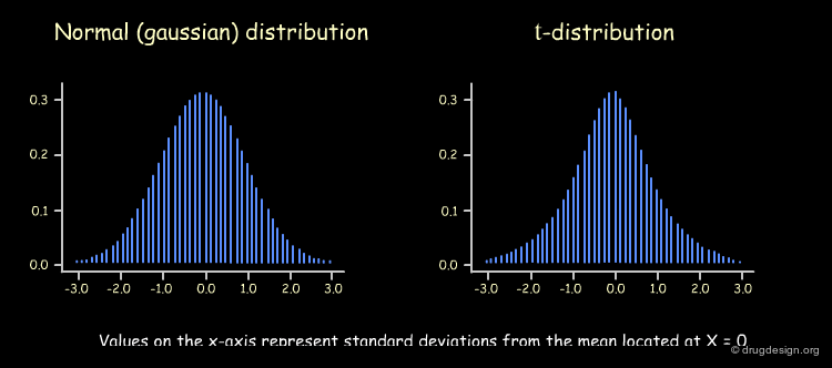
Shape of t-distribution and Number of Molecules
A value r2 = 1 will always be obtained for a set of two molecules irrespective of the descriptor used for the QSAR analysis however, as the number of molecules increases, the probability of obtaining large r2 values with irrelevant descriptors decreases. This probability corresponds to the area under the t-distribution curve (see below), away from the center (where r2 = 0). The shape of the t-distribution therefore depends on the number of molecules used in the analysis.

Student's t-test Procedure
The Student t-test employs the t-distribution to test whether the correlation coefficient obtained from the QSAR analysis is significantly different from 0. The larger the t-value, the larger the probability that r2 significantly differs from 0; that is, the larger the probability that the descriptor used for the analysis is relevant to the activity. Technically, the steps involved in the Student t-test are as follows.


F-test for Assessing the Significance of r2
The F-test is an extension of the t-test for the case of many descriptors. Like the t-test it tests (and hopefully rejects) the assumption that the model did not explain any of the original variance in the data set (i.e., ESS = 0). Like the t-test, the F-test uses an F-distribution which, similar to the t-distribution depends on the number of compounds and descriptors.

Performing the F-test
The F-test employs the F-distribution to test whether the correlation coefficient obtained from the MLR analysis significantly differs from 0. The larger the F-value, the larger the probability that r2 significantly differs from 0; i.e. the greater the probability that the descriptor used for the analysis is relevant to the activity. Technically, the steps involved in the F-test are as follows.

F-test Procedure
The application of the steps involved in evaluating the significance of r2 for the Capsaicin analogs using the F-test proceeds as follows:


Assessing the Predictive Power of a Model
r2, t and F are indices that can be generated to evaluate QSAR results. However, these parameters basically only tell us about the ability of the QSAR model to reproduce the data from which it was derived and not its aptitude to predict the activities of new compounds. Two methods are presented in the following pages to estimate the predictive power of a QSAR model.

The Test Set Method
The first method is known as the "test set method" and consists of partitioning the initial data into two sets, a preferred strategy when a large set of compounds is available. The initial data set is randomly divided into two parts; the first one is used to build a QSAR model and the second one to validate this model.

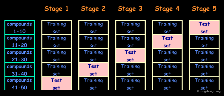
The Cross Validation Method
The second method is known as "the cross validation method" - it is preferred when the size of the data set is too small. In this method the data are randomly divided into N equal parts; N-1 parts are used to build the model which is then used for the remaining Nth part to predict the activities of the corresponding molecules. The procedure is repeated until the activities of all compounds have been predicted independently.
Limits of the Cross Validation Method
With the cross validation method, the QSAR model that is ultimately used to predict the activities of new compounds is derived from all N data points and is therefore different from the N partial QSAR models (i.e. those derived from the N-1 data points). Therefore cross validation does not provide us with the predictive power of a specific QSAR equation but rather with an estimate of our ability to make predictions for compounds similar to those used in our QSAR analysis.

The Predictive Index Q2
The predictive power of the model, termed Q2, is computed by analogy with r2, the difference being the use of the PRESS (predicted sum of squares) rather than the RSS (residual sum of squares) in the numerator. PRESS is calculated as the difference between the measured activity and the predicted activity for the test set compounds.

Summary
When discussing mathematical tools available for assessing the quality of a QSAR model we saw that (1) the standard deviation is an isolated "absolute" index of local meaning; (2) with r2 it is possible to compare different models, but this index is only mathematical - not statistical; (3) t and F have a statistical content that can be used for single and multiple linear regression respectively; however they only measure the ability of the QSAR model to reproduce the data from which it was constructed.
Copyright © 2024 drugdesign.org