3D-QSAR: Principles and Methods
Info
3D-QSAR is a method based on the analysis and the comparison of the 3D molecular fields (steric, electrostatic etc..) produced in the surrounding of different compounds for the establishment of a correlation between the biological activities and the fields. We present with some details CoMFA, the first approach developed and validated in the steroid area. The discipline has become mature and led to the development of new methods such as HASL, CoMSIA, CoMMA, MS-WHIM, SOMFA, HQSAR, GRIND, Quasar, CoMASA, Wep.
Number of Pages: 89 (±2 hours read)
Last Modified: January 2006
Prerequisites: QSAR Principles and Methods
Introduction
Molecular Binding Occurs in 3D
The biological activity of a ligand depends of its affinity with its receptor; this can be understood in molecular detail by identifying the interactions and forces involved in the binding process. Molecular binding occurs in 3D.

How Does the Receptor Perceives the Ligand?
The biological receptor does not see a ligand as a set of atoms and bonds, rather it perceives a shape that carries complex forces. In the 3D-QSAR framework these forces are considered to be determined predominantly by electrostatic and steric (van der Waals) interactions.

What is 3D-QSAR?
3D-QSAR is a method based on statistical correlation analyses enabling the comparison of 3D molecular forces ("fields") produced in the vicinity of different compounds to find correlations between biological activities and fields. This method generally applies in situations where the structure of the receptor is not known.

Principle of 3D-QSAR Approach
3D-QSAR is based on the mapping and the comparison of the steric and electrostatic fields around a set of ligands, to establish a 3D quantitative structure-activity relationship (3D-QSAR).

Intermolecular Forces
Electrostatic energy can be expressed as the inverse of the distance of the interacting atoms, whereas the steric energy depends on its inverse twelfth power. Thus, at long distances the electrostatic field drives the approach of the ligand to the active site, whereas at short ranges the steric forces become more important and control the final step of binding.

Electrostatic Field
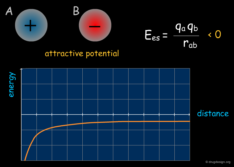
Electrostatic interactions occur between polar or charged groups. The electrostatic interactions between two molecules A and B are calculated as the sum of the interactions between point charges using Coulomb's law; they can be either attractive or repulsive. Since the electrostatic term can be expressed as the inverse of the distance, the electrostatic field is far from being negligible even when the groups involved are rather far apart (e.g. 10 angstroms or more).


Steric Field
The steric potential describes the non-electrostatic interactions between non-bonded atoms. The associated forces (called 'van der Waals' forces) can be either repulsive or attractive, depending on the distance between the atoms involved. At short distances, there is repulsion between atoms (due to the interpenetration of their electronic clouds), and at long distances, there is a small attraction (dispersion forces).

Difference between 2D-QSAR and 3D-QSAR
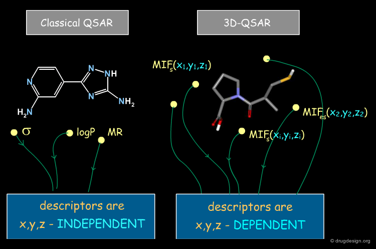
QSAR approaches aim to establish relationships between biological activities and chemical structure; however in classical QSAR molecular properties are described by parameters that are NOT x,y,z dependent (e.g. logP, MR, Es, Σ, π etc...), whereas in 3D-QSAR they are represented by a set of values of (x,y,z) functions, measured at many different locations in the space around the molecules. One consequence of this difference is that there are many more descriptors in 3D-QSAR than in classical QSAR.
Molecular Interaction Fields (MIF)
Interaction Field Surrounding a Molecule
Suppose that you have a molecule and a molecular property, for example the electrostatic field that can be calculated at any point from your molecule. The 3D distribution of the interaction field can provide relevant information concerning the properties of the molecule.

Perception of Interaction Fields
A field can be perceived only if there is a proper receiver able to interact with it. Take the example of the earth's magnetic field: you feel its existence if you have a compass, otherwise you cannot know if it exists. The situation is the same for molecular interaction fields: they can only be measured with the use of appropriate "probes"; this is discussed in the following pages.

Media
This picture was made using VMD and the APBS Plugin (electrostatic potential) APBS Tools
The Probe Concept
To test for the presence of a field and to measure it requires the use of probes with associated energy functions. Usually a probe atom is employed, which is placed at well selected points in the space, to quantitatively measure the value of the field created by the molecule at the point considered. The probe must be of the same type of the field to be measured (e.g. van der Waals probes for steric fields, charged probes for electrostatic fields).

Probing Steric Field with Single Atom Probe
The value of the steric field is calculated at different points in the space around a given molecule. The probe atom normally used to measure the steric field is a carbon sp3.

Probing Electrostatic Field with Single Atom Probe
The electrostatic field is measured at different points in the space around the molecule. The probe atom normally used is a carbon sp3 with a charge of +1.

Multi-Atom Probes
The probe concept has been extended to a whole range of molecular probes such as CH3, NH2, CONH2, H2O, NH3+ , COO- etc...
3D Lattice and Grid Points to Capture the MIFs
To simplify calculations of the fields created around a molecule, the method consists of superimposing a 3D lattice defining grid points regularly distributed in space, and calculating the interaction energy between the molecule and the probe at each grid point, using a potential energy function. The lattice makes it possible to sample the space with a finite number of points with MIFs that can be calculated in a reasonable amount of time.


Calculating the Electrostatic Field
The electrostatic field is obtained by calculating the electrostatic interaction energy between the molecule and the probe at each grid point using Coulomb's law.

Calculating the Steric Field
The steric field is obtained by calculating the van der Waals interaction energy between the molecule and the probe at each grid point using for example a 6-12 Lennard-Jones potential.

Visualization of MIFs with Iso-Potential Surfaces
Molecular interaction fields can be visualized by drawing iso-value surfaces around the molecule. An iso-value surface is a 3-dimensional surface connecting all points of the same value. In the course of a study many such surfaces are analyzed with the aim of deriving useful knowledge in structural terms.

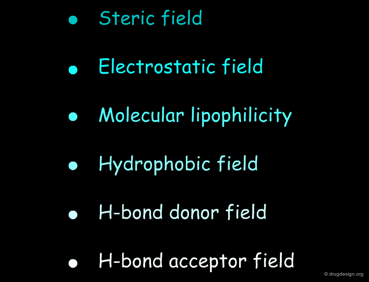
Other Molecular Interaction Fields
Besides the steric and electrostatic energies, other fields can be generated, depending on the probe and the potential energy function used to calculate the interaction. Additional fields include: interaction energies with functional groups, molecular lipophilicity field, hydrogen bond donor and hydrogen bond acceptor fields.
articles
HINT: A new method of empirical hydrophobic field calculation for CoMFA Kellogg, G. E.; Semus, S. F.; Abraham, D. J. J. Comput-Aided Mol. Des. 5 1991
3-D Molecular Lipophilicity Potential Profiles, A new Tool in Molecular Modeling P. Furet, A. Sele, N.C. Cohen Journal of Molecular Graphics 6 1988
Molecular lipophilicity potential by CLIP, a reliable tool for the description of the 3D distribution of lipophilicity: application to 3-phenyloxazolidin-2-one, a prototype series of reversible MAOA inhibitors Ooms F, Wouters J, Collin S, Durant F, Jegham S, George P. Bioorg Med Chem Lett. 8 1998
New Hydrogen-bond Potentials for Use in Determining Energetically Favourable Binding Sites on Molecules of Known Structure. Boobbyer, D.N.A., Goodford, P.J., McWhinnie, P.M. and Wade, R.C. J. Med. Chem. 32 1989
Comparative molecular similarity index analysis (CoMSIA) to study hydrogen-bonding properties and to score combinatorial libraries. Klebe, G.; Abraham, U. J. Comput.-Aided Mol. Des. 13 1999
The GRID Approach
The GRID Approach
The first program based on the calculations of MIFs was GRID, introduced by Peter Goodford in 1985 as a structure-based method to analyze the active sites of proteins.

articles
A Computational Procedure for Determining Energetically Favorable Binding Sites on Biologically Important Macromolecules. Peter J. Goodford J. Med. Chem. 28 1985
GRID: a Structure-Based Approach
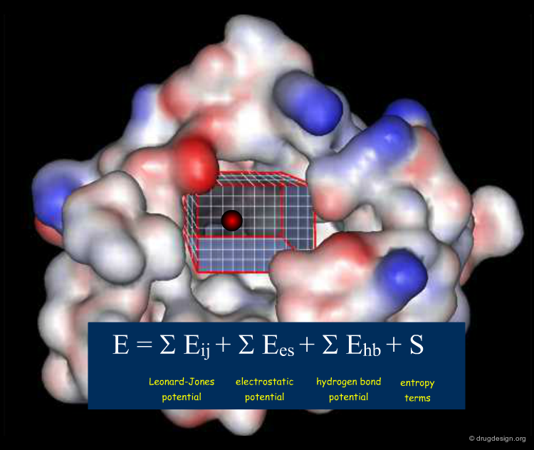
The active site is systematically explored by calculating the interaction energy between the protein and a chemical probe, at each grid point. A typical GRID interaction energy function between the protein and a probe is shown below.
Probing the Nature of the Active Site
Underlying the GRID approach is the idea that MIFs of different probes contain relevant information on the nature of the active site of a protein and the forces involved upon binding of a ligand.

The GRID Probes
Binding sites can be explored by using realistically shaped and charged probes. The GRID program contains several dozen probes such as a single atom, water, the methyl group, amine nitrogen, carbonyl oxygen, carboxylate and hydroxyl etc... More elaborate probes include metal cations (Na+, K+, Ca++, Fe++ , Fe+++, Zn++ , Mg++ ), aliphatic or aromatic (cis or trans) amides, aliphatic or aromatic cationic amidines, meta-diamino-benzene probes etc...

articles
New Hydrogen-bond Potentials for Use in Determining Energetically Favourable Binding Sites on Molecules of Known Structure. Boobbyer, D.N.A., Goodford, P.J., McWhinnie, P.M. and Wade, R.C. J. Med. Chem. 32 1989
Further Development of Hydrogen-Bond Functions for Use in Determining Energetically Favorable Binding Sites on Molecules of Known Structure. 1. Ligand Probe Groups with the Ability To Form Two Hydrogen Bonds Wade,R.C., Clark,K. and Goodford,P.J. J. Med. Chem. 36 1993
Further Development of Hydrogen-Bond Functions for Use in Determining Energetically Favorable Binding Sites on Molecules of Known Structure. 2. Ligand Probe Groups with the Ability To Form More Than Two Hydrogen Bonds Wade,R.C. and Goodford,P.J. J. Med. Chem. 36 1993
Integration of GRID with Other Programs
Initially the GRID program generated hundred of pages for each probe, with many tables listing the numerical values of interaction energies at each grid point, and the GRID MIFs proved to be of good quality. The advent of novel numerical statistical methods and progress in computer graphics have enabled the GRID output to be better analyzed.

Typical Use of GRID
GRID predicts favorable interaction positions ("hot spots") with the probes. When fragments are used as probes, the calculations reveal regions in the binding site where this fragment is likely to bind (see pyridine fragment illustrated in the view). This information can be exploited for the de novo design of new molecules.

articles
Rational design of potent sialidase-based inhibitors of influenza virus replication von Itzstein, M., Wu, W.Y., Kok, G.B., Pegg, M.S., Dyason, J.C., Jin B, Van Phan, T., Smythe, M.L., White, H.F., Oliver, S.W., et al. Nature 363 1993
'Flu' and Structure Based Drug Design Wade, R.C. Structure 5 1997
Outline of a GRID Calculation
The deployment of GRID requires: (1) the 3D coordinates of the atoms of the protein; (2) the binding site to be explored; (3) a selection of several probes; (4) run of GRID leading to the prediction of favorable positions for each probe; (5) analysis of the results with computer graphics.

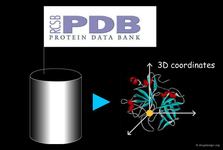
3D Coordinates of the Protein
The coordinates of the atoms of a protein are obtained from X-ray crystallography or NMR studies (the protein databank, PDB, is the most comprehensive source of high-quality 3D structures). For new proteins of known sequences, 3D models can be derived by homology modeling.
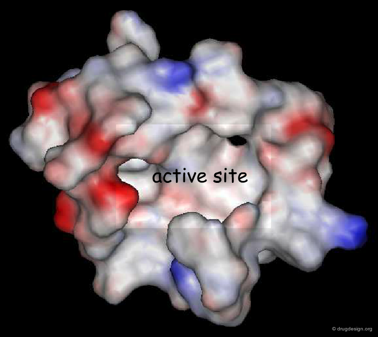
Binding Site to be Explored
The space surrounding the surface of a protein is huge and it is not necessary to explore the entire space. Normally the exact location of the binding site is known thus the calculation of the interaction fields can be limited to a box containing the active site to be explored.
Selection of Probes
Several dozen probes are available in GRID. The selection of the probes depends on the nature of the groups that are present in the binding site of the protein. One can address particular types of favorable energy interactions such as hydrophobic, aromatic, polar, salt-bridge interactions etc...

Run of GRID
For each probe and at each grid point of the lattice the molecular interaction fields are calculated. For multi-atom probes the probe is allowed to rotate at each grid point in order to find the lowest-energy orientation (e.g. essential for hydrogen bonding interactions), an optimization that is very demanding in terms of computing time.

Output of GRID
The GRID output consists of two types of files (line printer and binary) that need to be used in conjunction with other software. The binary files can serve as input for programs such as CoMFA, GOLPE, SIMCA for the statistical analysis of the GRID maps. Originally, when GRID was introduced visualization tools were not rich enough: advanced visualization programs only started to appear a few years later, enabling the effective visual interpretation of GRID results.

articles
Pattern Recognition by Means of Disjoint Principal Components Models Wold S Pattern Recognition 8 1976
book
Dunn W.J and Wold S. Chemometric Methods in Molecular Design VCH 1995
S. Wold and M. Sjoestroem ACS Symposium Series. Data Processing - Congress ACS 1977
Total Number of Calculations
The total number of GRID calculations is equal to the product of the number of compounds with the number of grid points and the number of probes. This must also be multiplied by the number of rotations, if several orientations at each grid point have been taken into consideration for multi-atom probes.

De Novo Design of New Scaffolds
GRID predicts favorable interaction positions with the probes and reveals where in the binding site a fragment of a given type will prefer to bind. Connecting a maximum of fragments in the correct orientation into a synthetically accessible molecule is not simple. Although GRID provides useful visual clues for creative structure design (de novo design), more advanced computerized approaches enable the systematic exploration of possible solutions (see design methods in chapters D2 and E2).

CoMFA: First 3D-QSAR Method
From GRID to 3D-QSAR
GRID is a MIF-based method developed for the analysis of macromolecule active sites, to reveal "hot spots" in their binding regions. It paved the way for the ideas that led to the development of the 3D-QSAR approaches, which retained the MIF concept and fully exploited it for the study of small molecule ligands, in projects where the 3D structure of the target protein is not known.
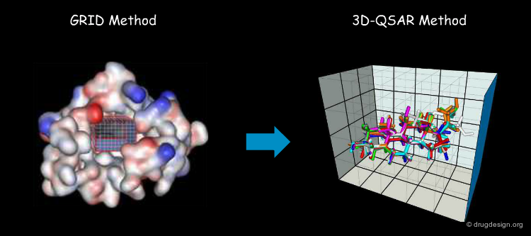
Comparative Molecular Field Analyses (CoMFA)
CoMFA is a method introduced by Cramer in 1988, for the COmparison of Molecular Field Analyses of different molecules. The method is based on the assumption that the 3D distribution of the interaction fields of a compound contains relevant information for understanding its biological activities. Comparison of the fields is expected to reveal important features concerning the activities of the molecules and can facilitate their optimization.

articles
Comparative Molecular Field Analysis (CoMFA). 1. Effect of Shape on Binding of Steroids to Carrier Proteins Richard D. Cramer III, David E. Patterson and Jeffrey D. Bunce J. Am. Chem. Soc. 110 1988
Development of a Correlation Function
Beyond the visual analysis of the MIFs of the active and inactive molecules, CoMFA aims at formulating a linear equation, correlating the biological activities with the values of the fields in each point. Here, each value calculated for a field on a given point (xi,yi,zi) is a descriptor.

Rapid Outline of a CoMFA Calculation
The development of CoMFA requires: (1) a set of related analogs; (2) defining a rule for superimposing them; (3) constructing a lattice of grid points and computing for each molecule the interaction with the probe at each point; (4) deriving a correlation function; (5) assessing the predictability of the model and (6) exploiting the results.

Reference Compounds and Initial Assumptions
A CoMFa study starts by selecting of a set of active/inactive molecules with their associated biological properties. Implicitly it is assumed that they share the same mechanism of action and that they are active for the same reason. All molecules are assumed to bind in the same way; it is also assumed that the biological action is enthalpically driven and that the entropic terms and desolvation energies are similar for all the compounds.

Superimpose the Structures
All molecules in the reference data set should be aligned to one another prior to the MIF calculation. Most typically used methods are based on the superimposition of their common chemical scaffolds or their common pharmacophores. Molecular alignment methods will be presented in more detail in the course of this chapter.

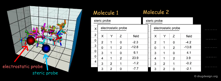
Calculate the MIF at Grid Each Points
First, a common lattice is constructed for the molecules superimposed. Then, for each separate molecule the molecular interaction fields are calculated for each probe and at each grid point. In CoMFA, only two probes are used: one for measuring the steric field and one for measuring the electrostatic field.
Derive a Correlation Function
The numerical values generated by the calculations are then processed by sophisticated mathematical statistical methods, with the aim of revealing a linear relationship between the field parameters and the biological activities. Normally the partial least-squares method (PLS) proves to be the method of choice in 3D-QSAR (statistical methods normally used in QSAR cannot handle the huge amount of data generated by CoMFA calculations).

Molecular Alignment Issues
Unfortunately CoMFA models are highly dependent on the way the molecules are aligned. The assumptions used in deriving alignments are therefore a difficult problem. Even for a series of related analogs, their exact orientation in the active site might be different (depending on the particular forces exerted by the protein on each ligand). The most common alignment methods are discussed in the following pages.
Template or Atom Alignments
A simple method consists of superimposing a set of atoms common to all the compounds. A molecule is chosen as a reference fixed template and the other molecules are moved to their new positions, corresponding to the minimum of the sum of the squared distances between a chosen set of atom pairs.
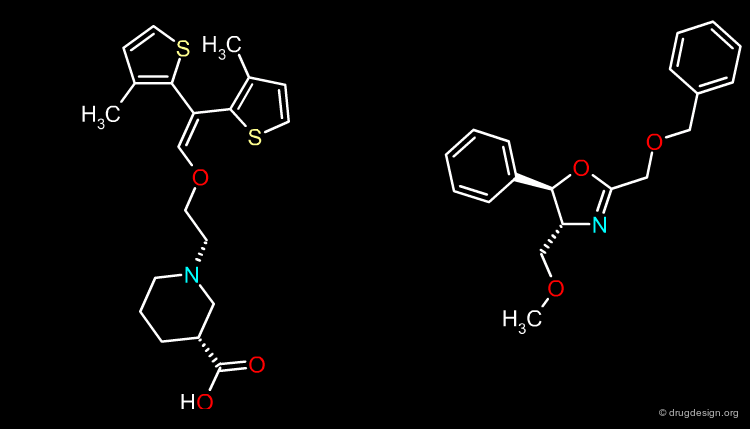
Pharmacophore Alignments
When there is no common scaffold shared by all the molecules it is possible to select pairs of atoms based on a common pharmacophore (or on chemical similarity assumptions). The molecules below illustrate a situation where the alignment of the molecules is not straightforward however this can be done by superimposing their common pharmacophore consisting of a fluoro-phenyl, an amino group and a carboxyl moiety.


Shape Alignments
In the absence of obvious rules, molecular modeling always enables the superimposition of molecules, based on shape alignments.

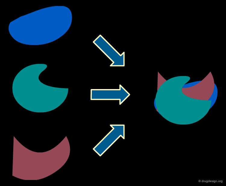
Field Fitting
After the steric and electrostatic fields around the molecules are calculated, it is possible to align the molecules by maximizing the overlap of the two fields. This method does not require the definition of any matching atoms.
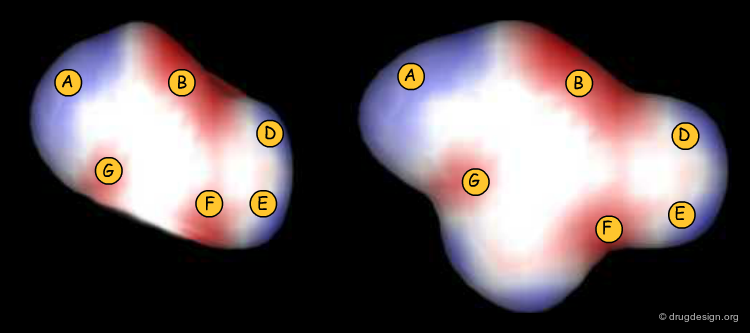
Electrostatic Field Alignment
This example from the EON program illustrates two chemically unrelated molecules (from MDDR) that could be superimposed by aligning the electrostatic fields created by the molecules in their vicinity (blue lobes are positive and red lobes are negative).

Moment Alignments
This is a less accurate alignment method; it consists of aligning the molecules based on molecular moments such as the molecular dipole, the principal moments of inertia or a field similarity moment.

articles
Computational methods for the structural alignment of molecules C. Lemmen and T. Lengauer Journal of Computer-Aided Molecular Design 14 2000
Three-Dimensional Moments of Molecular Property Fields B. David Silverman J. Chem. Inf. Comput. Sci. 40 2000
Comparative Molecular Moment Analysis (CoMMA): 3D-QSAR without Molecular Superposition B. D. Silverman and Daniel E. Platt J. Med. Chem. 39 1996
Receptor Based Alignments
The exact orientation of the molecules (from X-ray data or docking calculations with an homology model of the protein) would be ideal to have. Indeed, the position of each molecule in the active site depends on so many interactions that it would be excellent to conduct 3D-QSAR analyses where the orientation of the molecules is close to reality. This methods is only possible when the 3D structure of the receptor is known; however this is not the case in many CoMFA projects.

articles
Optimization of a pharmacophore model for 5-HT4 agonists using CoMFA and receptor based alignment Magdy N. Iskander, Lok M. Leung, Trevor Buley, Fadi Ayad, Juliana Di Iulio, Yean Y. Tan and Ian M. Coupar European Journal of Medicinal Chemistry 41 (1) 2006
A CoMFA study of COX-2 inhibitors with receptor based alignment Prasanna A. Datar, Evans C. Coutinho Journal of Molecular Graphics and Modelling 23 2004
Three-dimensional quantitative structure-activity and structure-selectivity relationships of dihydrofolate reductase inhibitors Jeffrey J. Sutherland and Donald F. Weaver Journal of Computer-Aided Molecular Design 18 2004
3D-QSAR CoMFA, CoMSIA studies on substituted ureas as Raf-1 kinase inhibitors and its confirmation with structure-based studies Ram Thaimattam, Pankaj Daga, Shaikh Abdul Rajjak, Rahul Banerjee and Javed Iqbal Bioorg Med Chem 12 2004
Alignment from X-ray Data
The following analogs are inhibitors of CP450-cam, and it is reasonable to assume that they bind to a sub-pocket having a shape corresponding to their common similar volumes. However X-ray studies reveal a somewhat different alignment of the three molecules (see button "X-rays").

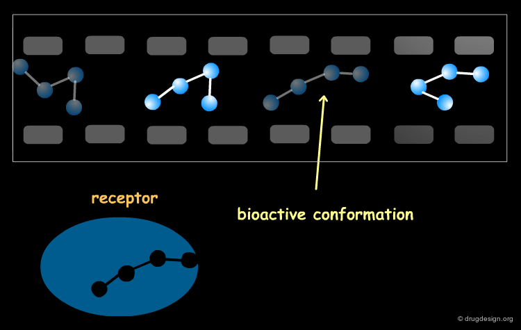
The Bioactive Conformation Issue
Bear in mind that whatever method is used for superimposing the molecules, they must be aligned in their bioactive conformations. Preliminary analyses are needed to establish these, and in some cases it may be necessary to consider several hypotheses. CoMFA studies are always safer with a set of homolog compounds. The historical CoMFA paper by Cramer was on steroid analogs, a case where the conformational "risk" was minimal.
articles
Multimode Ligand Binding in Receptor Site Modeling: Implementation in CoMFA Lukacova, V. and Balaz, S. J. Chem. Inf. Comput. Sci. 43 2003
QSAR of conformationally flexible molecules: Comparative molecular field analysis of protein-tyrosine kinase inhibitors Nicklaus, M. C.; Milne, G. W. A.; Burke, T. R., Jr. J. Comput.-Aided Mol. 6 1992
Modified CoMFA methods for the analysis of antineoplastic effects of lignan analogues Broughton, H. B.; Gordaliza, M.; Castro, M.-A.; Miguel del Corral, J. M.; San Feliciano, A. J. Mol. Struct.(THEOCHEM) 504 2000
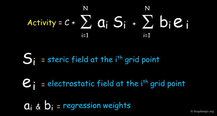
Deriving the 3D-QSAR Correlation Function
The aim of the 3D-QSAR is to derive a linear function, which predicts the biological activities of the molecules in terms of the individual values calculated for the fields (si and ei are the steric and electrostatic descriptors, respectively).

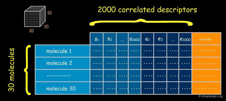
Problem of Number of CoMFA Descriptors
The number of descriptors accumulated in a CoMFA analysis (columns) is by far greater than those in a QSAR study (in classical QSAR the number of molecules exceeds the number of descriptors by a factor of 3-5, whereas in CoMFA, the number of descriptors exceeds the number of molecules by a factor of several thousand). Moreover, the descriptors are highly correlated because many of the values of neighboring grid points are similar. Classical QSAR regression techniques (e.g. MLR) cannot be employed with this type of data.
PLS: the Partial Least-Squares Method
The statistical method known as Partial Least Squares (PLS) has proven to be suited for handling this complex multivariate problem by eliminating the correlation between the descriptors, reducing their number and enabling the generation of a linear relationship between the field parameters and the biological activities.

articles
PLS-regression: A basic tool of chemometrics Wold, S.; Sjostrom, M.; Eriksson, L. Chemom. Intell. Lab. Syst. 58 2001
Sample-distance partial least-squares PLS optimized for many variables, with application to CoMFA Bush, B. L.; Nachbar, R. B. J. Comput.-Aided Mol. Des. 7 1993
Generating optimal linear PLS estimations (GOLPE): an advanced chemometric tool for handling 3DQSAR problems. Baroni, M.; Constantino, G.; Cruciani, G.; Riganelli, D.; Valigi, R.; Clementi, S. Quant.Struct.-Act. Relat. 12 1993
book
Wold S, Albano C, Dunn WJ, Esbensen K, Hellberg S, Johansson E, Sjstrm M Food Research and Data Analysis Applied Science 1983
Wold S Methods and Principles in Medicinal Chemistry Vol 2. Verlag Chemie 1995
Wold S, Albano C, Dunn WJ, Edlund U, Esbensen K, Geladi P, Hellberg S, Johansson E, Lindberg W, Sjstrm M Chemometrics: Mathematics and Statistics in Chemistry Reidel 1984
Geometrical Interpretation of PLS
Consider a case where we want to predict the activity for n molecules using values of 3 descriptors (X1,X2,X3). PLS aims at reducing the initial referential to a space of reduced dimension and generating a reduced set of variables t (the t's being a linear combination of the original X's). In the example below, the 3D space has been reduced to 1D where the biological activities are predicted in a simple linear fashion, activity = ct.

The First PLS Component
The first PLS component (t1 axis) is a line in the initial X-space which satisfactorily approximates the points in terms of least squares and at the same time provides a good correlation in the t-space.

The Second PLS Component
The second PLS component (t2 axis) is a line orthogonal to the first PLS component, which correctly approximates the points in the (t1,t2) plane, and at the same time provides an improved correlation in the t-space. Subsequent PLS components are derived in a similar manner.

3D-QSAR Equation in the PLS Space
Thanks to the reduction of the number of terms by PLS calculations, an equation in the form of a linear relationship between structure and activity is obtained. Note that the new variables "ti" do not have a structural meaning.

Back to Space of Original Descriptors
The 3D-QSAR PLS equation is a good mathematical model, with however a poor structural content. To circumvent this drawback, this equation is projected back into the space of the original descriptors, to yield an equivalent CoMFA equation that can be better exploited in structural terms.

The 3D-QSAR Equation in the Original Data Space
The CoMFA equation consists of a linear combination of Si (the steric field) and ei (the electrostatic field) calculated at each point of the lattice. This equation can be used to highlight regions in space where steric or electrostatic interactions are critical for the activity, and this will be presented a few pages later.
Many Terms in the 3D-QSAR Equation
Unlike classical QSAR equations that can be clearly written, 3D-QSAR equations never appear explicitly. This equation contains thousands of terms, each of which is associated to a particular (xi,yi,zi), which is impossible to represent in a linear expression. The CoMFA equation can be fully assessed and exploited however its linear form remains in the computer. The number of terms collected in the data space may be 25.000-55.000, depending on the number of molecules, the lattice dimension and spacing. PLS analyses can reduce them by a factor in the range of 4 to 40.

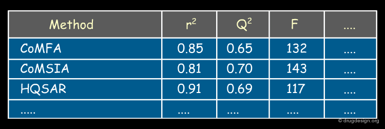
Measuring the Quality of the Relationship
The indexes used for assessing the quality of a 3D-QSAR model are the same as those already presented for the classical QSAR regression model: r2 (squared correlation coefficient); TSS (total sum of squares), ESS (explained sum of squares), RSS (residual sum of squares), SDEP (standard deviation in error prediction), Fvalue (F-test of statistical significance), q2(cross-validated correlation coefficient) provide measures of the degree of correlation between the activity values calculated by the model and those measured experimentally. Usually different models are envisaged and these numbers serve to assess their respective quality and predictability.

articles
Beware of q2! Golbraikh A, Tropsha A. J Mol Graph Model. 20 2002
PLS-regression: A basic tool of chemometrics Wold, S.; Sjostrom, M.; Eriksson, L. Chemom. Intell. Lab. Syst. 58 2001
Sample-distance partial least-squares PLS optimized for many variables, with application to CoMFA Bush, B. L.; Nachbar, R. B. J. Comput.-Aided Mol. Des. 7 1993
Generating optimal linear PLS estimations (GOLPE): an advanced chemometric tool for handling 3DQSAR problems. Baroni, M.; Constantino, G.; Cruciani, G.; Riganelli, D.; Valigi, R.; Clementi, S. Quant.Struct.-Act. Relat. 12 1993
Comparative Study of 3D-QSAR Techniques on Angiotensin II Receptor (AT1) Antagonists P. A. Datar, E. C. Coutinho and Sudha Srivastava Letters in Drug Design and Discovery 1 2004
book
Wold S Methods and Principles in Medicinal Chemistry Vol 2. Verlag Chemie 1995
Wold S, Albano C, Dunn WJ, Edlund U, Esbensen K, Geladi P, Hellberg S, Johansson E, Lindberg W, Sjstrm M Chemometrics: Mathematics and Statistics in Chemistry Reidel 1984
Total Number of PLS Components
The method known as 'cross validation' is used to fix the total number of PLS components (axis). The calculations are repeated with a randomly chosen set of compounds, and the resulting model is used to predict the missing activity data. Q2 is the correlation between the measured activities and the predicted ones. New PLS components are added as long as Q2 continues to increase.

Two Equivalent 3D-QSAR Equations
We now have two equivalent 3D-QSAR equations: the first one is the PLS equation (in the t-space), and the second is the projection of the first in the space of the original descriptors. The former is useful for numerical calculations, and the later for 3D visualizations to provide insight into the structural content of the resulting 3D-QSAR model.

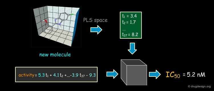
Predicting the Activities of New Compounds
Once a model is formed it can be used to predict the biological activity of a molecule which has yet to be synthesized and tested. The same sequence is repeated: alignment, interaction fields and projection in the PLS space to predict its activity. If a designed molecule is structurally new, care must be taken when aligning it with the reference compounds.
CoMFA Coefficient Contour Maps
Thanks to the back-projection of the PLS equation into the space of the original data, the resulting equation can be exploited for the construction of CoMFA contour maps. A typical contour map is created by connecting points of the 3D grid with similar favorable or unfavorable coefficient values of a given field, multiplied by the standard deviation. The visualization of the contour map highlights regions where interactions are critical for activity. In the example below, point P2301 contributes sterically to 0.1% of the activity.


CoMFA Steric Contour Map
In the example below a steric coefficient contour map is visualized, on top of a reference molecule. Green and yellow contours (a color code now widely adopted) indicate regions where bulky groups increase or decrease activity, respectively.

CoMFA Electrostatic Contour Map
Electrostatic contour maps are constructed in a similar manner, and can be visualized with a now widely adopted color code. Blue contours indicate regions where electropositive groups increase activity, whereas red contours represent regions where electronegative groups increase activity.

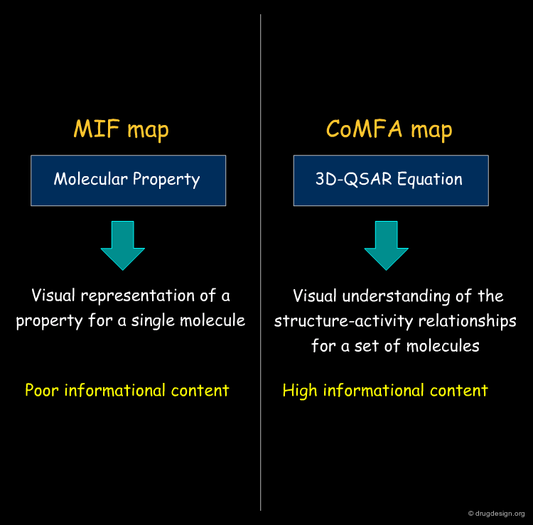
CoMFA Contour Maps vs. MIF Contour Maps
The CoMFA maps help understand the SAR, give an idea of the nature and the regions where interactions with the receptor are critical, and also to exploit them for designing new molecules. These maps have high informational content, contrary to MIF iso-potential maps that only visualize a molecular property, with no relationship whatsoever with the biological effects.
Analysis of Steric Contour Maps
The visual analysis of a CoMFA steric map is straightforward. One can recognize regions where steric interactions with the receptor are favorable (green regions) or unfavorable (yellow regions). It is easy to imagine what kind of analogs are likely to be more potent or less potent than the reference compound.

Analysis of Electrostatic Contour Maps
A ComFA electrostatic contour map reveals critical regions: the blue areas correspond to regions where electronegative groups decrease activity and electropositive groups increase activity; by contrast red areas correspond to regions where electronegative groups increase activity and electropositive groups decrease activity. One can imagine what kind of analogs are likely to be more potent or less potent than the reference compound.

Exploitation of the Steric Contour Map
In the example below, when bulky para substituents are introduced in the phenyl ring pointing towards the green area, biological activities are increased; whereas para substitution of the second phenyl ring is detrimental to these activities.

Exploitation of the Electrostatic Contour Map
When electronegative groups (Cl, CF3) are introduced into the red areas biological activities are increased; and when electronegative groups (Br, CN) are in the blue areas biological activities are decreased.
Stability Problem of CoMFA Models
CoMFA models are sensitive to the parameters used to construct them. For example, very small changes in the relative alignment of the molecules can result in substantially different regression models. Other parameters include the lattice (spacing, orientation and dimensions) or the methods used for calculating the fields. The stability of the models is a difficult issue which is explicitly addressed by the new methods currently in development.
articles
On the Stability of CoMFA Models James L. Melville and Jonathan D. Hirst J. Chem. Inf. Comput. Sci. 44 2004
Predictive Binding of beta-Carboline Inverse Agonists and Antagonists via the CoMFA/GOLPE Approach Allen M. S.; LaLoggia A. J.; Dorn L. J.; Martin M. J.; Constantino G.; Hagen T. J.; Koehler K. F.; Skolnick P.; Cook J. M. J. Med. Chem. 35 1992
Replacement of steric 6-12 potential-derived interaction energies by atom-based indicator variables in CoMFA leads to models of higher consistency Kroemer R. T.; Hecht P. J. Comput.-Aided Mol. Des. 9 1995
A Different Method for Steric Field Evaluation in CoMFA Improves Model Robustness Sulea T.; Oprea T. I.; Muresan S.; Chan S. L. J. Chem. Inf. Comput. Sci. 37 1997
Finding Optimum Field Models for 3D QSAR Kellogg G. E. Med.Chem. Res. 7 1997
The Effect of Region Size on CoMFA Analyses Bucholtz E. C.; Tropsha A. Med.Chem. Res. 9 1999
A Benchmark Set for 3D-QSAR
The introduction of CoMFA triggered the development of an entire generation of new 3D-QSAR methods, which will be presented in the next section.

articles
The CoMFA Steroids as a Benchmark Dataset for Development of 3D QSAR Methods Coats, E. A. Perspectives in Drug Discovery and Design 12/13/14 1998
The Thirty-one Benchmark Steroids Revisited: Comparative Molecular Moment Analysis (CoMMA) with Principal Component Regression B. David Silverman Quantitative Structure Activity Relationships 19 2000
Other 3D-QSAR Methods
3D-QSAR Programs
After the introduction of CoMFA, other 3D-QSAR methods were developed by different groups. Some of these programs are mentioned below, listed by first date of publication. In the following pages the specificity of some of them is briefly outlined.

Best Method?
It is not unusual to see QSAR practitioners simultaneously using several methods, comparing the corresponding models with the statistics associated to them, for purposes of deciding which method is the most suitable for their particular application. An objective comparison among methods is still not possible, in particular because of the stability problem mentioned previously. Many research groups have their favorite method and keep one or two data sets to validate new ones they develop.
articles
Comparative Study of 3D-QSAR Techniques on Angiotensin II Receptor (AT1) Antagonists P. A. Datar, E. C. Coutinho and S. Srivastava Letters in Drug Design and Discovery 1 2004
Three-dimensional quantitative structure-activity relationship analyses of a series of cinnamamides Tingjun Hou and Xiaojie Xu Chemometrics and Intelligent Laboratory Systems 56 2001
A Comparison of Methods for Modeling Quantitative Structure-Activity Relationships Jeffrey J. Sutherland, Lee A. O'Brien and Donald F. Weaver J. Med. Chem. 2004 47 2004
A CoMFA study of COX-2 inhibitors with receptor based alignment Prasanna A. Datar, Evans C. Coutinho Journal of Molecular Graphics and Modelling 23 2004
CoMFA
The CoMFA approach (comparative molecular field analysis, developed by R. Cramer et al.) uses steric and electrostatic fields to capture the properties of the space around a molecule. The probe atom is a carbon with a charge of +1. CoMFA paved the way for the development of several generations of new 3D-QSAR methods.

articles
Comparative Molecular Field Analysis (CoMFA). 1. Effect of Shape on Binding of Steroids to Carrier Proteins Richard D. Cramer III, David E. Patterson and Jeffrey D. Bunce J. Am. Chem. Soc. 110 1988
HASL
In HASL (hypothetical active site lattice, developed by A. Doweyko et al.) a molecule is converted into a set of regularly-spaced points (lattice) defined by Cartesian coordinates (x,y,z) and atom type. In this way individual molecules can be compared to one another, and their lattices merged to form a composite description called the HASL. The individual property of each molecule is distributed among the points in the HASL in such a way that the sum of the partial activity values associated with a set of points belonging to each molecule is equal to the total known value for that molecule. The result is a model of the receptor site consisting of points in space capable of predicting the activities of new molecules.

articles
The Hypothetical Active Site Lattice. An Approach to Modelling Active Sites from Data on Inhibitor Molecules Arthur M. Doweyko J. Med. Chem. 31 1988
CoMSIA
The CoMSIA approach (comparative molecular similarity index analysis, developed by G. Klebe et al.) uses molecular potentials that are smoothed with Gaussian functions to eliminate singularities at atomic nuclei (as observed in CoMFA). This has been proven to reduce the sensitivity to small changes in the alignment of compounds or the orientation of the grid. In addition to the steric and electrostatic fields CoMSIA includes hydrogen bonding (donor and acceptor) and hydrophobic fields.

articles
Molecular similarity indices in a comparative analysis (CoMSIA) of drug molecules to correlate and predict their biological activity Klebe, G.; Abraham, U.; Mietzner, T. J. Med. Chem. 37 1994
Comparative molecular similarity index analysis (CoMSIA) to study hydrogen-bonding properties and to score combinatorial libraries. Klebe, G.; Abraham, U. J. Comput.Aided Mol. Design 13 1999
CoMMA
CoMMA (comparative molecular moment analysis, developed by D. Silverman et al.) is a method based on descriptors such as the moments of inertia, dipole and quadrupole moments, that do not require molecular superposition or alignment for the assignment of molecular similarity. Initially developed for properties where the zero-order moment of the expansion vanishes, the approach has been extended to cases where this is not true, and higher levels of moment expansions of property fields are then considered (first-order, second-order moments).

articles
Three-Dimensional Moments of Molecular Property Fields B. David Silverman J. Chem. Inf. Comput. Sci. 40 2000
MS-WHIM
MS-WHIM (molecular surface weighted holistic invariant molecular, developed by G. Bravi et al.) is a method based on a small number (e.g. 12) of statistical parameters derived from molecular surface properties and calculated within different weighting schemes. The MS-WHIM fields contain structural information in terms of size, shape, symmetry and atom distribution that are invariant with respect to the coordinate system.

articles
MS-WHIM, new 3D theoretical descriptors derived from molecular surface properties: A comparative 3D QSAR study in a series of steroids Gianpaolo Bravia, Emanuela Ganciaa, Paolo Mascagnia, Monica Pegnaa, Roberto Todeschinib and Andrea Zaliania Journal of Computer-Aided Molecular Design 11 1997
SOMFA
SOMFA (self-organizing molecular field analysis, developed by D. Robinson et al.) is an approach where the fields are calculated as in CoMFA however their values are multiplied by the activity of the molecule expressed on a scale where the most active molecules have positive values and the least active molecules have negative values. Therefore the most active and least active molecules have higher values than the less interesting ones, which are close to the mean activity. This form of descriptor filtering intends to increase the quality of the correlation.

articles
Self-Organizing Molecular Field Analysis: A Tool for Structure-Activity Studies Daniel D. Robinson, Peter J. Winn, Paul D. Lyne, and W. Graham Richards J. Med. Chem. 42 1999,
HQSAR
In the HQSAR method (Hologram-QSAR, developed by T. Heritage et al.) the structure of a molecule is encoded as a single string of binary numbers. The different molecular substructures are expressed in fingerprints that are then hashed into hologram bins and used as descriptors in QSAR models. A molecular hologram contains all the possible molecular fragments within a molecule and implicitly encodes 3D structural information. The method is somewhat related to the early Free-Wilson approach in which activities are correlated with the presence of various functional groups.

book
Heritage, T. W.; Lowis, D. R. Rational Drug Design: Novel Methodology and Practical Applications Oxford University Press 1999
GRIND
GRIND (GRid-INdependent descriptors, developed by G. Cruciani et al.) is a method producing descriptors that are calculated from the 3D structure of the molecules, but they do not depend on their position or orientation in the space. In the first step several fields are calculated and transformed (simplified), and in the second step the results are encoded into alignment-independent variables based on auto-correlation theory. The results can be visualized with 2D or 3D diagrams.

articles
GRid-INdependent Descriptors (GRIND): A Novel Class of Alignment-Independent Three-Dimensional Molecular Descriptors Manuel Pastor, Gabriele Cruciani, Iain McLay, Stephen Pickett and Sergio Clementi J. Med. Chem. 43 2000
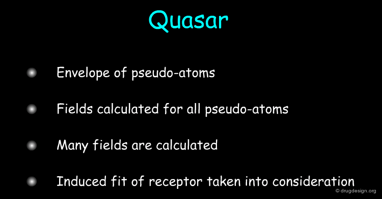
Quasar
The Quasar approach (quasi-atomistic SAR, developed by A. Vedani et al.) is based on the construction of an envelope of pseudo-atoms that represent the surface of a putative binding site. Several fields are calculated for each of these pseudo-atoms; they include hydrophobic neutral, salt bridge positive, salt bridge negative, H-bond donor, H-bond-acceptor, hydrophobic positive, hydrophobic negative, H-bond flip/flop, solvent fields. Induced-fit of the receptor to the different compounds is taken into account by allowing the mean envelope to adapt its shape to the individual molecules.
articles
Quasi-atomistic receptor modeling. A bridge between 3D QSAR and receptor fitting Vedani A and Zbinden P. Pharm Acta Helv. 73 1998
CoMASA
CoMASA (comparative molecular active site analysis, developed by T. Kotani et al.) is a method replacing the 3D regular grid points of the lattice by a small number of "representative points" selected by cluster analysis (tree-variable multivariate). No alignment of the molecules is needed and the method is very rapid (e.g. for the 31 steroid benchmark, only 92 representative points are sufficient, instead of the 7200 grid points normally used in CoMSIA).
articles
Comparative molecular active site analysis (CoMASA). 1. An approach to rapid evaluation of 3D QSAR Takayuki Kotani and Kunihiko Higashiura J Med Chem. 47 2004
WeP
WeP (weighted probes, developed by W. Shin et al.) is based on the idea that certain regions of the receptor surface contribute, to varying extents, to the differences in the activities of the ligands, whereas other regions do not. The probes, placed around the surface of a superimposed set of ligands, are associated with fractional weights, which are then optimized with a genetic algorithm. A pseudo receptor is generated, which consists of the surviving probes with nonzero weight values.

articles
Novel Receptor Surface Approach for 3D-QSAR: The Weighted Probe Interaction Energy Method Chong Hak Chae, Sung-Eun Yoo, and Whanchul Shin J Chem Inf Comput Sci. 44(5) 2004
Conclusion
Conclusion
3D-QSAR proves to be very useful for the optimization of a reference chemical structure by improving the binding affinities with an unknown receptor. The method generates data of great practical value such as correlation functions and 3D visualizations of favorable and unfavorable interactions with the receptor. 3D-QSAR is a tool that holds a great potential and is expanding rapidly towards a broader field of application.

Copyright © 2024 drugdesign.org