Molecular Dynamics
Info
This chapter deals with Molecular Dynamics (MD) and its applications to the study of complex molecular systems. The aim of the chapter is to introduce basic concepts and algorithmic issues behind MD, as well as practical simulation protocols and MD packages. Examples of problems that can be explored using MD and specific MD simulations are discussed, with the goal of illustrating the current state-of-the-art in this field. After reading this chapter, the reader should have a better understanding of how MD can be used to study molecular systems, as well as how to set up and run MD simulations and analyze the resulting trajectories.
Number of Pages: 143 (±3 hours read)
Last Modified: September 2006
Prerequisites: None
Introduction
What is Molecular Dynamics?
Molecular Dynamics (MD) is a method developed to reproduce and understand the behavior of molecular systems. It is a statistical mechanics approach for simulating complex systems. The on-going revolutionary advances in computer technology and algorithmic improvements have made MD a valuable tool in many areas of physics and chemistry, including studies on the structure and dynamics of macromolecules, such as proteins and nucleic acids.

articles
Molecular dynamics simulations of biomolecules M. Karplus and A. McCammon Nature Structural Biology 9 2002
wikipedia
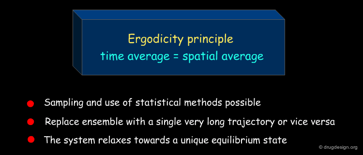
Ergodicity Assumption
MD simulations are based on the ergodicity assumption, which makes it possible to use statistical methods. The ergodicity assumption states that the ensemble average is equal the time average. As a consequence the average value does not depend on initial conditions and the system relaxes towards a unique equilibrium state.
Historical Note
Molecular Dynamics emerged as one of the first computer simulation protocols in the late 1950s. The first MD simulations were the pioneering applications to the dynamics of liquids by Alder and Wainwright and by Rahman. MD simulations of proteins started to appear in the early 1970s, as exemplified by the pioneering works of McCammon and Karplus. Today a large number of research groups are actively involved in the development of this field.

articles
Molecular dynamics simulations of the complete satellite tobacco mosaic virus. Peter L. Freddolino, Anton S. Arkhipov, Steven B. Larson, Alexander McPherson, and Klaus Schulten Structure 14 2006
Nanoseconds molecular dynamics simulation of primary mechanical energy transfer steps in F1-ATP synthase R.A. Boeckmann and H. Grubmueller Nature Structural Biology 9 2002
Phase transition for a hard sphere system Alder, B. J. and Wainwright T. E. J. Chem. Phys. 27 1957
Studies in molecular dynamics: General methods Alder, B. J. and Wainwright T. E. J. Chem. Phys. 31 1959
Correlation in the motion of atoms in liquid Argon A. Rahman Phys. Rev. A 136 1964
Improved simulation of liquid water by molecular dynamics Stillinger, F. H. and Rahman A. J. Chem. Phys. 60 1974
Dynamics of Folded Proteins McCammon, J. A., Gelin, B. R., and Karplus M. Nature 267 1977
Four Types of Applications of MD Simulation
Molecular Dynamics simulation methods can be used for four different purposes. They can be used: (1) to study the dynamical behavior of a system; (2) to calculate the properties of a system at equilibrium (e.g. thermodynamics); (3) as a tool for sampling the different configurations of a system; (4) for structure refinement in conjunction with experimental data.

Macroscopic Behavior
Information about macroscopic behavior can be obtained from a simulation of a system at the atomic level. Let's revisit the notion of "atoms in molecules" and inter-atomic interactions that lay the foundation for the MD approach to atomistic simulations.

MD Between Experiment and Theory
Science progress is made through experiment, theory and, as of the last 50 years or so, simulation. Computer simulation approaches such as MD have altered the interplay between experiment and theory. The essence of a simulation is the use of the computer to model physical systems. Complex calculations projected by a mathematical model are actually carried out by a computing device and the results are interpreted in terms of physical properties. Computer simulations enable physical quantities to be in a sense measured on a computer; hence, the term "computer experiment".

Refinement and Validation of MD
Biomolecules are studied through a variety of experimental techniques that help reveal their structure and dynamics, interactions with other molecules, physical and chemical properties, etc. In particular, X-ray crystallography, NMR spectroscopy and electron microscopy are used to reveal the structure of large biomolecules and their complexes with atomistic resolution. That enables better parameterization of models used in MD and direct comparison between simulation and experiment.

Access to Unavailable Data
On the other hand, bottlenecks and limitations on experimental structure determination make computational methods a valuable alternative to experimental techniques.

MD Applied to Living Systems
While MD can be applied to any complex system, this chapter focuses on biological systems that are built and maintained by an array of molecules: proteins, nucleic acids, lipids etc. MD often leads to new insights into mechanisms and processes that are not directly accessible through experiment. Three examples are presented in the following pages that illustrate the molecular machinery of life and the relationships between structure and function.

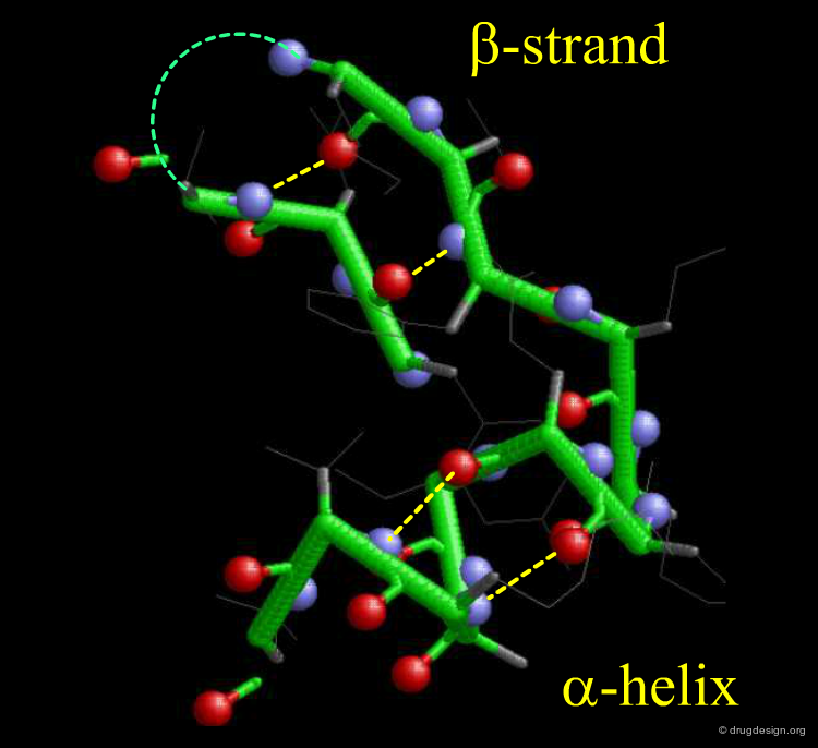
Example 1: Relation between Structure and Function
Proteins perform their functions by adopting certain three-dimensional structures which typically consist of specifically arranged secondary structure elements. Idealized backbone conformations for alpha helical and beta sheet secondary structures are visualized in the figure below. Note the existence of hydrogen bonds and other non-covalent interactions that are important in stabilizing these conformations (side chains and water molecules are not shown for simplicity).
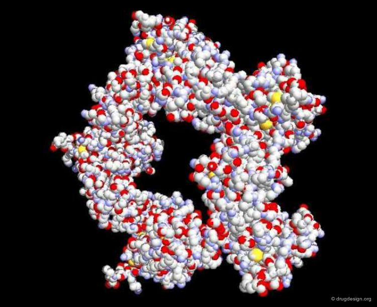
Example 2: Relation between Structure and Function
Annexin is an alpha helical protein that forms oligomeric complexes that are capable of dissolving lipid membranes of pathogens. Understanding atomistic interactions between annexin and phospholipids is important for controlling (and understanding) its function.
wikipedia
Example 3: Relation between Structure and Function
RNA Polymerase II is a major transcription enzyme which is shown here in a complex with DNA (white) and transcribed RNA (green). Specific interactions play a central role in stabilizing the transcriptional transition state where complementary mRNA is built from DNA templates.

wikipedia
Proteins are not Static
The 3D structure of a system helps determine its properties; however a static 3D representation may not be sufficient for understanding systems such as those mentioned in the previous pages because proteins are not static and remain in continual motion. Studying protein movement, including thermal fluctuations and conformational changes, brings essential insights into structure-function relationships.
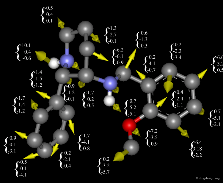
Thermal Fluctuations
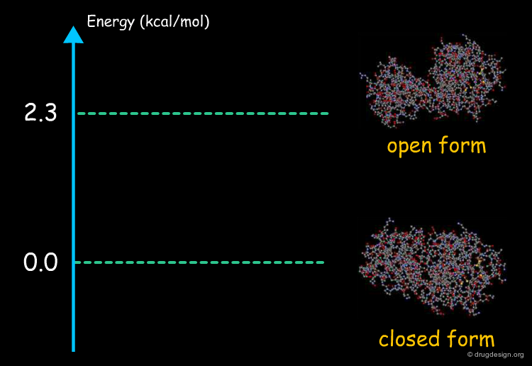
Real molecules "breathe" due to thermal fluctuations. These thermal motions are inherent to all chemical processes, and to the "structure" and function of molecular systems. Thermal fluctuations can be studied using MD. In the example below, thermal fluctuations of a protein are illustrated. As can be seen from the movie, thermal fluctuations can lead to inter-conversion between distinct conformations separated by low energy barriers.

Conformational Changes
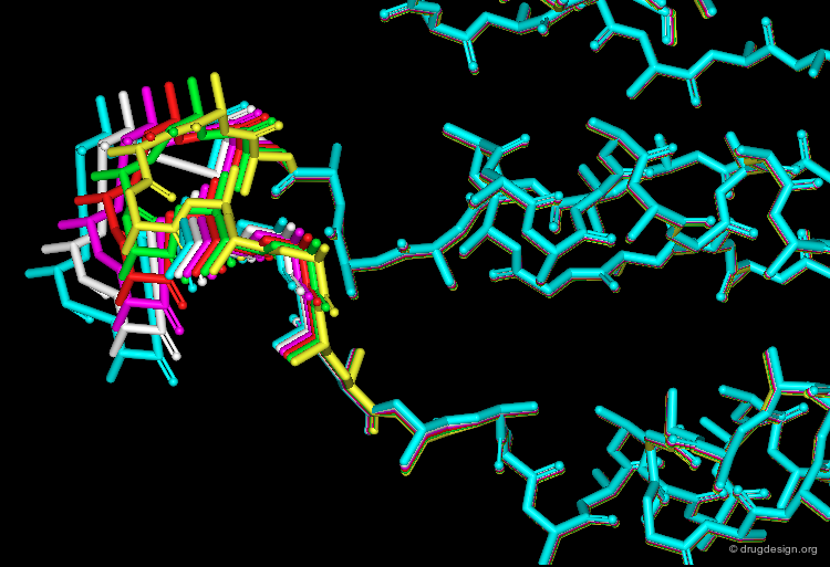
In addition to thermal fluctuations, there are also large scale conformational changes that are observed both experimentally and via simulation. The example below illustrates conformational changes in the "MAD2 spindle assembly checkpoint" protein induced by ligand binding. MD simulates the interconversion between unbound (blue) and bound state (yellow).
MD as a Way to Study Molecular Motions
MD provides a means to study the molecular motions of a system by determining how it will move by calculating the trajectory of the atoms.

Mimicking the Way a Molecule Moves
Molecular dynamics mimics the way a molecule explores its conformational space. The models generated by MD are closer to reality than the static structures obtained by other methods (e.g. molecular mechanics).
Average Properties Derived from MD Trajectories
Knowing the motion over time of a system makes it possible to derive its properties and observables by using concepts in statistical mechanics, where physical quantities are represented by averages over microscopic states (configurations) of the system, as a function of a certain statistical distribution. A physical quantity can therefore be measured by taking an arithmetic average over instantaneous values of that quantity obtained from MD trajectories.

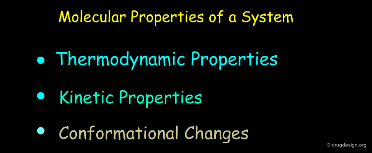
Calculating Molecular Properties of a System
Examples of properties that can be calculated include average energies, temperature factors etc... More generally, thermodynamic and kinetic properties as well as conformational changes are important molecular features that can be derived from MD trajectories, as explained in the following pages.
Studying Thermodynamic Properties
By studying thermal fluctuations around local minima by using MD we can derive the thermodynamic properties of the system. The information obtained about the motion of the individual atoms can be condensed and methods in statistical mechanics can be applied to deduce thermodynamics properties of the system such as entropy, Gibbs free energies, enthalpy, binding energies, specific heats etc...

articles
Thermodynamic calculations in biological systems L. Mario Amzel, Xavier Siebert 1, Anthony Armstrong, German Pabon Biophysical Chemistry 117 2005
Studying Kinetic Properties
Kinetic properties can be calculated using MD simulations. Folding rates for the villin headpiece protein have been estimated successfully using MD. Repeated attempts to fold a protein from its extended conformations are required to estimate folding rates, making the problem computationally very expensive.

Studying Conformational Changes
One of the most crucial questions in structural biology is how a protein chain can spontaneously fold into a highly ordered three-dimensional structure in spite of the vast number of possible conformations. This is known as the protein folding problem, and can be studied using molecular dynamics.

Energy Calculations
Calculation of Forces & Energies
Computation of forces and energies of a molecular system are of central importance in MD because they control and dictate the detailed dynamics of the system. In the following pages we introduce the concept of "atoms in molecules" (quantum mechanics) and atomistic force fields (molecular mechanics) that enable the calculation of the energy of a molecular system.

Two Families of MD Methods
In MD simulations, energies (and in particular the potential energy), can be calculated either with first-principle approaches (quantum mechanics) or by treating the molecules as classical objects resembling the 'ball and stick' model (molecular mechanics). These two approaches define the two families of MD treatments.

The Quantum Mechanics Approach
The quantum or first-principles MD simulations (first introduced by Car and Parinello) explicitly take into account the quantum nature of the chemical bond. The electron density function for the valence electrons that determine bonding in the system is computed using quantum equations, whereas the dynamics is determined classically.

wikipedia
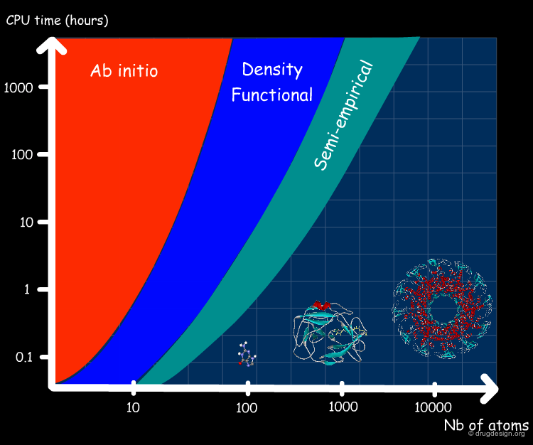
Quantum Methods are Computationally Expensive
Quantum MD simulations are computationally very expensive since they involve estimation of electron density in each step. Ab-initio, density function and semi-empirical methods are all quantum mechanical methods based on the Schrodinger equation.
The Classical Mechanics Approach
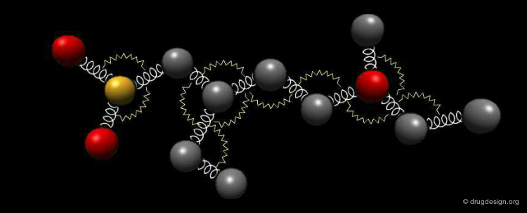
In the classical mechanics approach to MD simulations, molecules are treated as classical objects where atoms correspond to soft balls and bonds are represented by elastic sticks with parameters chosen to approximate their true (and quantum in nature) characteristics. The problem of finding a realistic potential that can adequately mimic the true potential energy surfaces results in major computational simplifications. The laws of classical mechanics are used to describe the dynamics of the system. In the following, we will focus on classical MD.
wikipedia
Classical vs. Quantum Methods
Classical mechanics ("force field") calculations are much less computationally expensive than quantum mechanical methods.

Classical MD Simulates the Dynamics of the Nuclei
Classical MD simulates the dynamics of the nuclei but electrons are not present explicitly in the treatment. The nuclei move on a potential energy surface, and electrons are indirectly introduced through this surface that is solely a function of the atomic positions. The non-explicit account of the electrons is justified by the Born-Oppenheimer approximation that is explained on the next page.

The Born-Oppenheimer Approximation
The Born-Oppenheimer approximation is based on the fact that nuclei are much heavier than electrons (e.g. the carbon nucleus has a mass over 20,000 times that of the electron). As a consequence the nuclei move more slowly than the electrons and the electron clouds "equilibrate" quickly for each instantaneous configuration of the heavy nuclei.

wikipedia
Force Field for Classical MD
In classical MD the potential energy is calculated by a molecular mechanics model, an approach based on the idea that the atoms of the molecule feel forces and the energy of a given configuration is related to these forces. An empirical set of energy functions called force field enables the simulation of such forces.

wikipedia
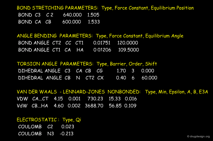
General Force Field Equation
The expression of the potential energy is indicated in the formula below. The first three terms run over all the bonds, angles and torsion angles defined by the covalent structure of the system, whereas the last two terms run over all the pairs of atoms (or sites occupied by point charges), separated by distances and not bonded chemically. Each term of the force field will be presented in the following pages.
wikipedia
Stretching Term
Physically, the first term describes deformation energies of the bond lengths with respect to their equilibrium values. The harmonic form of these terms (with force constant ai ) insures a correct chemical structure; but on the other hand, it restricts modeling chemical changes, as it does not allow for the breaking of bonds, for instance.
Bending Term
The second term describes deformation energies of the bond angles with respect to their equilibrium values. The harmonic form of these terms (with force constant bi ) insures correct chemical structure.

Torsional Term
The third term describes rotations around chemical bonds, which are characterized by periodic energy terms (with periodicity determined by n and heights of rotational barriers defined by ci ). The γi constant enables the shift of the curve along the Ω axis.

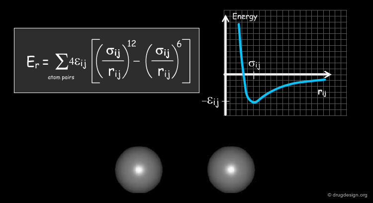
Van der Waals Term
The fourth term describes the Van der Waals repulsive and attractive (dispersion) interatomic forces in the form of the Lennard-Jones 12-6 potential. Attractive dispersion (Van der Waals) interactions result from polarization of electron clouds; their range is significantly shorter than that of electrostatic interactions. Short range Van der Waals interactions represent the repulsion between electron clouds due to the exclusion principle. A 1D Lennard-Jones potential curve (with its parameters Σ and {epsilon} ) is depicted below.
Electrostatic Term
The last term is the Coulomb electrostatic potential. Some effects due to specific environments (e.g. polarizability) can be accounted for by properly adjusted partial charges and an effective value of the constant k.

A Couple of Practical Remarks
Different MD packages may use different functional forms of the force field (e.g. the Van der Waals parameters may be derived differently from atomic parameters, some force fields may include explicit polarization terms etc.). Moreover, the final choice of parameters typically results from fitting to different experimental data. Therefore, individual parameters, such as partial charges, are in general not transferable between different force fields. Due to specific parameterization, some force fields may be better suited for studying specific problems (e.g. kinetic vs. thermodynamic aspects or nucleic acids vs. lipids, etc.).

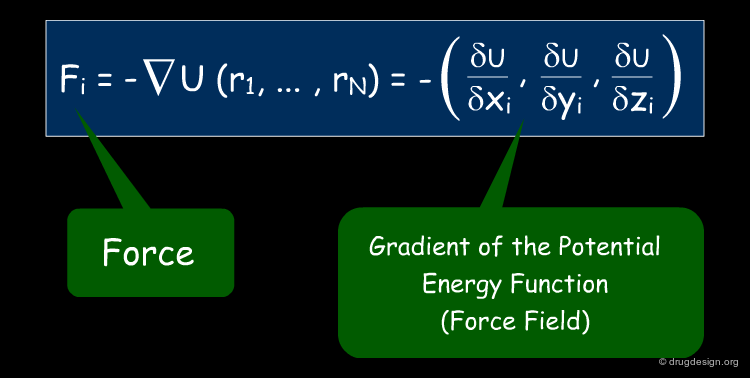
The Link between Forces and Potential Energies
In MD we need to know the forces exerted on each atom. These forces are calculated as the gradient (first derivative) of the energy function U(r1, ..., rN) with respect to atomic displacements. The link between forces and potential energies is shown in the equation below, where U characterizes the potential energy of the system (which is approximated by the force field).
MD Algorithm
Newton's Equation of Motion
We are now ready to define the molecular dynamics algorithm, which is at the core of MD simulations. It is based on Newton's equation of motion, the fundamental equation of classical mechanics which relates the force acting on a body to the change in its momentum over time : F=ma ("F" is the force exerted on the particle, "m" is its mass and "a" is its acceleration).

Prediction of Next Position
Newton's equation of motion is used to propagate the nuclear coordinates of the molecular system in time. Using (1) the forces exerted on the atoms (derived from the force field), (2) the atomic coordinates and (3) the velocities, it is possible to solve the equations of motion and obtain the next position of the configuration in space.

Integration Step
MD advances the system by one integration step and generates a new configuration at each step. The numerical integration of the equations of motion requires discretization of the equations with a finite time step Δt, which is called the "integration step". We will later see that Δt needs to be very small in order to produce reliable results.

Molecular Dynamics Algorithm
A molecular dynamics simulation starts by assigning some kinetic energy to each atom in the system. This initial kick causes the molecules to move around. It is possible to predict how the system will move in the very near future by solving Newton's equations. Using the values of atomic forces and masses of the system at time t, solving these equations will give the positions of each atom at time (t+Δt).

Trajectories: List of Positions and Velocities
The MD simulation consists of a succession of predictions on how the system will move over time. This is represented by a series of snapshots called trajectories. The MD trajectories are defined by both position and velocity vectors and they describe the time evolution of the system.

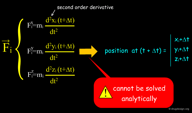
Atomic Positions at Time (t+Δt)
The purpose of solving Newton's equations is to calculate the atomic positions at time (t+Δt) in terms of positions which are already known at time t. This requires solving a set of differential equations.

Solving Newton's Equations
For a system consisting of N atoms, Newton's equations represent a set of 3N second order differential equations. In current (many-body) systems these equations cannot be solved analytically. Instead, approximate solutions are used where the equations are discretized and solved numerically. One method is presented on the next page.
Numerical Integration with the Verlet Formula
One commonly used method of numerical integration of motion was first proposed by Verlet which computes atomic positions at time t+Δt from the forces and positions at previous times. Note that velocities are not included in the Verlet formula, but they can be derived from the atomic positions. Many other methods have been devised and employed in MD simulations for solving Newton's equations, but the Verlet algorithm remains popular because of its simplicity and stability.


Summary of the MD Algorithm
The MD algorithm is summarized here. It starts by assigning initial positions and velocities to all the atoms. A loop starts where forces exerted on each atom at the current time are calculated and Newton's equations of motions are solved for all the atoms over a short time step Δt. Current trajectories are then stored and the loop is repeated for a new time (t+Δt). The process is complete when the time scale has been entirely covered.

Fundamental Issues
Time Step
The calculations of motion are done at discrete intervals; the length of these intervals defines the time step. The time step must not be too short - to achieve sufficient sampling, and not too long - to avoid jeopardizing the stability of the system. The choice of the time step of a MD simulation is an important issue that is discussed on the next page.

Choice of Time Step
To correctly capture the motions we want to analyze, the time step must be small in comparison to the highest frequency motion in the molecule. Therefore a time step of 1 femtosecond is generally used, because it is one order of magnitude less than the fastest motions (bond stretching and bond angle vibrations).

Time-Scale of Molecular Motions
Current molecular dynamics can examine systems on time scales in the order of nanoseconds. With a time step of 1 femtosecond, a million integration steps are needed to provide just a nanosecond of simulation. Move the cursor over each type of motion to see the number of cycles needed to simulate the corresponding motion. For example, fast protein folding occurs in 10 µs and would require 109 cycles.

Method for Increasing the Time Step: Constrained MD
One way to increase the time step and by extension the sampling of longer time scales, is to use a constrained MD to eliminate the fastest motions from the system. For example, the so-called SHAKE algorithm is widely used to effectively fix fast vibrating bonds and angles at their equilibrium values. However, even if the fastest vibrations are filtered out, a time step of more than 5 fs is difficult to achieve in MD simulations.

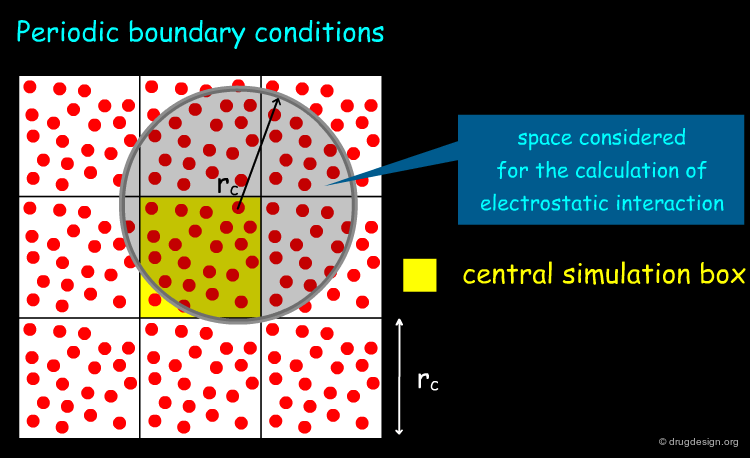
Periodic Boundary Condition
MD simulations are designed to predict the overall properties of a system and not its surface effects. Surface effects are eliminated using the so called "periodic boundary conditions" which consists of replicating the simulation box to form an infinite 3D lattice. Over the course of the simulation, when any atom or molecule moves in the central box, its periodic image in the other boxes moves in exactly the same way. Therefore when an atom leaves the central box, one of its images enters through the opposite face. Since there are no "walls" at the boundary of the central box, the system has no surface.


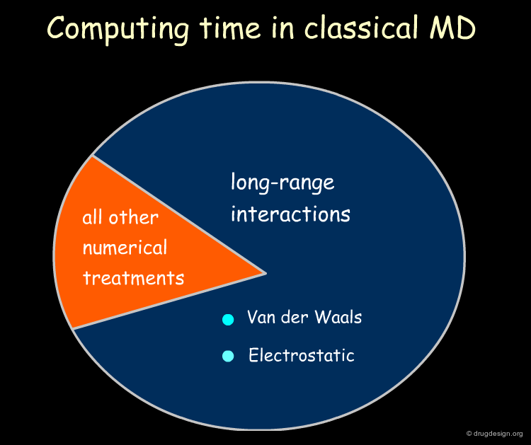
Importance of Long Range Forces
Long range forces such as electrostatic and dispersion interactions are known to play an important role in biomolecules. The proper treatment of these interactions has become one of the most important issues in this field. Accounting for these interactions, involves a summation over all pairs of atoms in the system. When the number of such pairs is high (e.g. above 10,000), a huge bottleneck is created, affecting the computer time needed to calculate them in MD simulations.

articles
On the truncation of long-range electrostatic interactions in DNA. Norberg, J., and L. Nelsson. Biophys. J. 79 2000
Effect of electrostatic force truncation on interfacial and transport properties of water. Feller, S. E., R. W. Pastor, A. Rojnuckarin, S. Bogusz, and B. R. Brooks. J. Phys. Chem. 100 1996
Dynamical Properties of a Hydrated Lipid Bilayer from a Multinanosecond Molecular Dynamics Simulation Preston B. Moore, Carlos F. Lopez, and Michael L. Klein Biophys. J. 81 2001
Molecular dynamics free energy simulations: Influence of the truncation of long-range nonbonded electrostatic interactions on free energy calculations of polar molecules C. Chipot, C. Millet, B. Maigret and P.A. Kolmann J. Chem. Phys. 101 1994
The Distance Cutoff Concept
In order to reduce the computing time in MD a distance "cutoff" concept has been introduced. The idea consists of truncating the long range (electrostatic and dispersion) interactions and not calculating them beyond a given distance threshold.


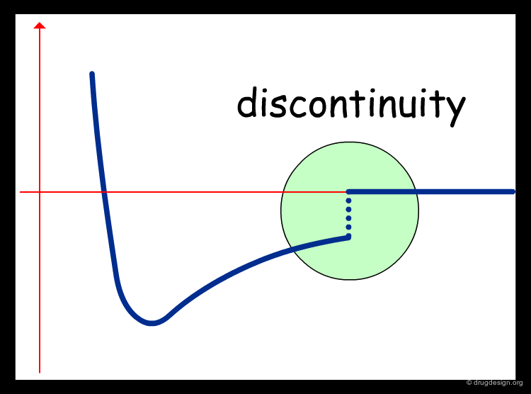
Problems with Cutoffs
A cutoff distance unavoidably introduces a discontinuity because up to the cutoff value the energy function is used, and beyond, the interaction energy becomes zero. Such an abrupt discontinuity has been shown to create problems in the stability of the system and the energy of the system is not conserved.
Switching Functions
One way to circumvent this difficulty is to introduce a "switching function" that will smoothly decrease the interaction energy from the value calculated at a "switch distance" (point A) on the energy function, to point B (cutoff distance) for which the switching function becomes zero.
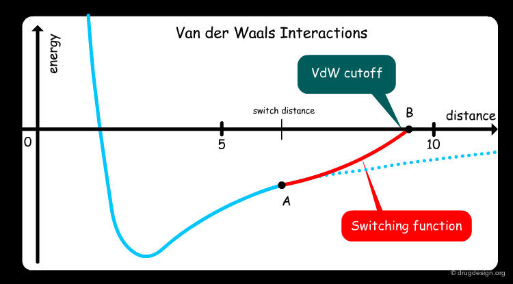
Choice of the Cutoff
The dilemma is that the computational effort in the MD algorithm is dominated by the repeated calculations of all the instantaneous long range forces in the system, whereas neglecting them leads to inaccurate models. Since detailed studies show that long range interactions are crucial to both the dynamics and the structural simulation it is necessary to assign sufficiently large values to the cutoffs. For example 8-10 Å for dispersion interactions and 11-15 Å for electrostatic interactions.

Strategies to Incorporate the Solvent
This dilemma prompted the development of several strategies to incorporate the solvent in MD simulations. Both implicit and explicit solvent models have been developed, and this is presented on the next pages.

Implicit Solvent Model
Implicit solvent models treat water as a continuous medium by approximating the free volume available as a continuum with average properties such as electrostatics, dielectric constant and entropic properties that match real water.

Explicit Solvent Molecules
Explicit solvent models represent thousands of water molecules explicitly. Such solvent models are more accurate, but also more expensive computationally. For example, when using a box of 50x50x50 Å3 one needs about 10,000 water atoms and more than 92% of the time is spent on the calculation of water-water interactions. There are however, many efficient approaches to computing long range forces for explicit solvent models, such as the Ewald method presented on the next page.

The Ewald Summation Method
The Ewald summation method has long been applied in the simulation of liquids and was transposed recently to the treatment of biomolecular systems (see scheme below). Although imposing an artificial periodicity in the system, the Fast Fourier Transform-based Particle Meshed Ewald (PME) method enables accurate summation of electrostatic and long range interactions without resorting to crude cutoff approximations. This method is nowadays routinely used in MD for the calculation of long range forces.
MD Protocols
Typical Steps for MD Simulation
In the following section we provide details on the protocol to set up MD simulations up to the production runs. The steps involved include: (1) the preparation of the system; (2) the choice of the program; (3) the assignment of values to the parameters of the simulation; (4) preprocessing (e.g. equilibration) and finally (5) the launch of the MD simulation. This is presented on the following pages.
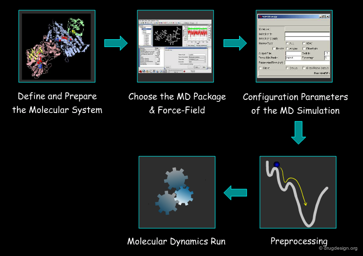
Define and Prepare the Molecular System
The first step in MD simulations involves defining the chemical structure of the system, which is typically represented in terms of individual (predefined) molecules and "monomers" for biological polymers, such as proteins and nucleic acids.

Preparing the Coordinates
Initial coordinates of the system may be obtained in a variety of ways. If a relevant structure is known, then all one needs to do is to download it from the Protein Data Bank, Cambridge Crystallographic Database or another resource. When no experimental data can be used (e.g., when attempting to fold a protein from an extended conformation), the initial set of coordinates may be constructed using chemical and physical principles as a guideline.

Manual Assembly of a Complex Molecular System
One outcome of the increase in computational power is that molecular dynamics studies of complex and large biological systems are now feasible. Such systems are generally not experimentally available and are constructed by the manual assembly of their different components.
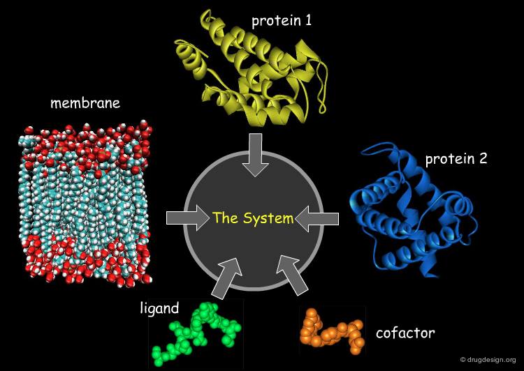
Solvating the System
A solvation model is necessary to better simulate the biological environment of the system. If an explicit solvation model is adopted (which is preferred and more accurate than the continuum solvation model) the system needs to be solvated by water molecules. There are many ways to solvate a molecular system, with or without boundary conditions. For example, the system can be placed in a water sphere, or in a water box within the framework of periodic boundary conditions.

Addition of Counterions
When there is a charged protein, it is typical to add charge-balancing counterions to the solution to neutralize the system. For example if we have a protein with either charged acidic residues (e.g aspartic or glutamic acids) or with charged basic residues (e.g. arginine or lysine residues) counterions such as Ca+, Na+, Cl- can be used and placed in idealized positions (energy minima) to balance the corresponding charges. Not every charged residue requires a counterion, since these may be involved in salt bridge interactions.

Choose the MD Package & Force-Field
For most macromolecules (proteins, nucleic acids, sugars, lipids and other biomolecules) force field parameters are in principle already available. Packages such as AMBER or CHARMM were extensively checked against many such systems and have well documented strengths and weaknesses. The program that best fits the problem at hand should be used.

Extending the Parameterization of the Force Field
For small molecules or ligand binding studies some force field parameters may be missing. In such a case, equilibrium geometries, partial charges and other parameters may be obtained using quantum chemical programs such as GAUSSIAN. Extending the force field to new entities is not always easy, and care should be taken to verify the consistency of such defined parameters with the rest of the force field.
Configuration Parameters of the MD Simulation
The next step in the preparation of a MD run is to define the simulation parameters. The most important ones include the definition of the time step, the length of the simulation, distance cutoffs, frequency for updating the list of non-bonded atom pairs, initial velocities and possible parameters for geometrical constraints.

Time-step
A time step is specified, usually in femtoseconds, to define the quantity to be used in the numerical integration for each step of the simulation.

Length of the Simulation
The number of simulation time-steps to be performed in the MD simulation is defined by the user who stipulates the total time for the simulation. A total time of 500 picoseconds is a very short time indeed in MD; however it has been shown that this may be qualitatively sufficient for many problems.

Distance Cutoffs
The distance cutoffs to be used in the simulation are introduced in the input. One cutoff distance is defined for the Van der Waals interactions, and another one for the electrostatic interactions.

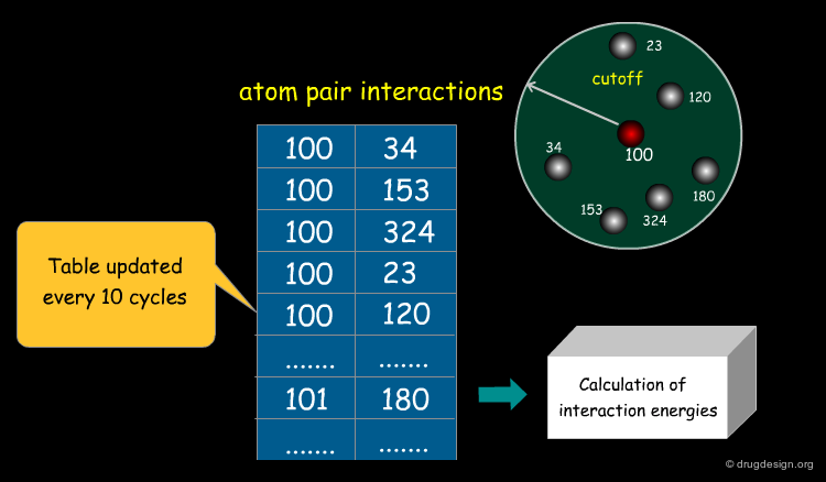
Reassigning the List of Non-Bonded Atom Pairs
Because important conformational changes do not occur rapidly, the list of all pairs of atoms for which non-bonded interactions should be calculated (having their distance within the cutoff) is updated only periodically (e.g. after 10-15 steps) and not after each iteration. This contributes to reducing the time for calculating non-bonded interaction energies.
Initial Velocities
Initial velocities need to be given for each atom in order to initiate a MD simulation. Theoretically a file can be filled in with the desired values; however in this case the set of values must correspond to the desired temperature for the system. A more convenient alternative for assigning atomic velocities consists of specifying a temperature; the program will then distribute initial velocities using a simple Maxwell-Boltzmann distribution equation. One can also progressively heat the system.
SHAKE Parameters
We saw that the SHAKE algorithm allows you to increase the time step by fixing bond lengths or angles at their equilibrium values. For example all the bonds of the system, or all O-H bonds, or all water molecules can be assigned a fixed geometry. Each of these options is indicated by the user in the SHAKE parameter input. By default the system is not constrained at all, and free to move.

Preliminary Treatments: Minimization & Equilibration
The next step in the MD simulation involves energy minimization followed by thermal equilibration of the system. Although minimization and equilibration seem similar, they differ in the way they use the force field. Energy minimization consists of successive alterations of the geometry of the system until a minimum is found on the conformational potential surface whereas equilibration is driven by Newton's equations of motion that dictate to the structure which pathways to follow on that surface.
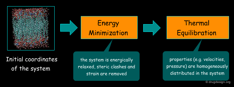
Minimization of Initial Coordinates
The system with its initial coordinates is subjected to an energy minimization. This treatment is necessary because there might be steric clashes (e.g. when the system is built from scratch) resulting in a "blow-up" of the energy function. The minimization brings the structure to one local minimum of the potential surface. Being consistent with the overall definition of the force field, the system is now at 0oK temperature.

Thermal Equilibration of the System
The system needs to be equilibrated thermally before running the actual simulations. Equilibration consists of a MD run in which the temperature is gradually increased from zero to the final temperature (typically around 300oK, corresponding to physiological conditions). The quality of the equilibration is assessed by how well velocities fluctuate around average values and implies that they are well distributed over a given amount of time. In practice the thermal equilibration involves heating and equilibration using the Maxwell-Boltzman equation, as explained on the following page.

Maxwell-Boltzmann Equation
The Maxwell-Boltzmann equation (formula 1) is a random Gaussian distribution often used to assign initial values to the velocities in the thermal equilibration and to assess the stability of the system during the simulation. The magnitude of the velocities is chosen for the required temperature and corrected so there is no overall momentum (formula 2). The temperature can be calculated from the velocities using the equation indicated below (formula 3).


wikipedia
Molecular Dynamics Run
Following its thermal equilibration, the system is ready for the production runs. Multiple MD trajectories may be generated from the initial (equilibrated) configuration. Furthermore, sampling different initial states by choosing alternative initial geometries and equilibration procedures may help achieve overall better sampling and convergence of the simulations.

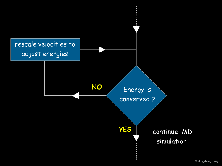
Conservation of the Total Energy
MD treatments generally simulate isolated systems. However, the energy of a MD simulation is not always strictly conserved. This occurs when cutoff distances are too small, when the time step is too large, or if the precision of the computer is not sensitive enough.

Test Energy Fluctuation
Estimating the fluctuation of energy is a good test of the quality of MD simulations. Tricks of the trade, like changing the parameters of the run or occasional rescaling of velocities, may need to be used to adjust the energy, making a thorough equilibration of the system an important issue.
Possible Crash of the Program
Even with the best of luck, the instabilities of numerical integration of the equations of motion may cause the program to crash from time to time. Trajectories may be carefully restarted in such cases, but attention should be paid to the sources of these problems. In many cases, cut off simulations with an explicit solvent may add to such instabilities and considering PME (see Ewald method) as an alternative approach may help limit energy fluctuations and numerical instabilities.

Analysis of the Results of the MD Simulation
Analysis of the Results
Hopefully the MD simulation has terminated successfully and we can now derive a great deal of information from the huge amount of data generated. All intermediate structures with their detailed atomic coordinates, velocities, energies etc... are stored and ready to be exploited. Special programs and their combinations are used to extract specific information such as average properties (energies, thermodynamic and kinetic properties), structural information (local and global conformational changes). This is presented on the following pages.

Thermodynamic Properties
Now that we have the trajectories, we can address questions such as: what states are possible? what states are "visited"? In particular the pathway of interconversion between two conformations is a key piece of information about the function of a protein that can be revealed by a MD simulation.
articles
Thermodynamic calculations in biological systems L. Mario Amzel, Xavier Siebert 1, Anthony Armstrong, German Pabon Biophysical Chemistry 117 2005
Kinetic Properties
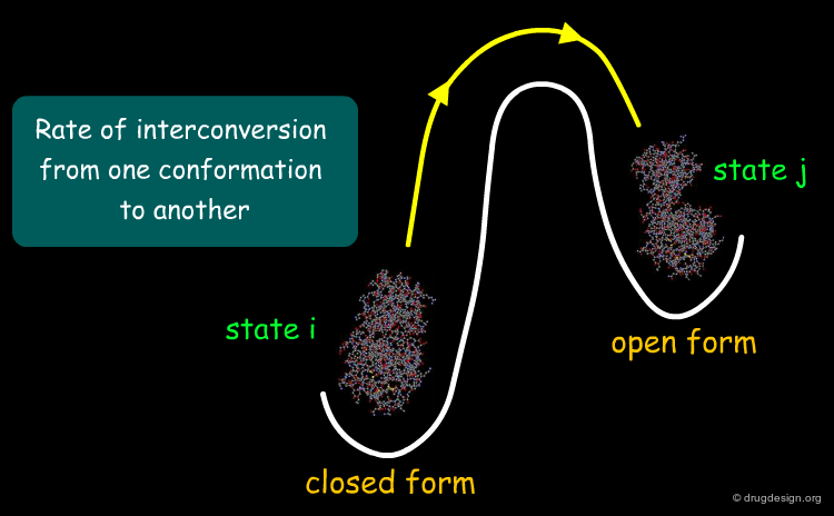
The kinetic energies can be calculated over the course of the simulation and we can follow the system's trajectory when it interconverts between states. Kinetic features can also be analyzed by deriving various quantities of interest, such as specific distances or presence of secondary structure elements that may indicate sudden conformational changes. For example one can assess how fast interconversions occur and the rates of such processes.
Visualization of Time Dependent Properties
Time dependent properties can be visualized graphically where the x-axis represents the time and the y-axis the quantity of interest (e.g. a distance, a torsion angle, the energy, atomic fluctuations, radius of giration etc...). In addition, the time dependent variation of the Φ-Ψ torsion angles of a given residue can be represented graphically with a Ramachandran plot for this particular residue.


Deriving Average Properties from the Trajectory
Analysis of the trajectories often involves computing averages over instantaneous values of the quantity of interest, as obtained from MD trajectories. Coordinates and velocities of the system are used for these calculations. Examples of average properties calculated from MD simulations are presented on the following pages.

Average Energies
Energies are of central importance in a MD run, and it is possible to calculate either the average total energy or one of its components (e.g. dispersion or electrostatic interactions) for the whole system or for one individual moiety.
Specific Heat
The specific heat of the system (e.g. protein in solution) can be easily calculated. To do so, it is necessary to extract the total energies for the atoms in the system and apply the formula shown below, which needs both the average and the squared-average total energy.

wikipedia
Radius of Gyration
The radius of gyration measures the compactness of the structure that is commonly traced during simulations. Its value for a particular geometry or as an average (throughout the full range of conformations) is calculated by the mass weighted scalar length of each atom from the center-of-mass using the formula shown below.

Local Motions
The RMS deviation over time of the residues of a protein can be useful to analyze. The MD run makes it possible to generate a table of all residues with their associated RMS deviations; however a graphic representation of this property is sometimes much preferred. For the protein represented below, the backbone is displayed and color coded by the value of the RMS deviation of each residue.

Interesting Motions
Over a short period of time (e.g. a fraction of a picosecond), molecular dynamics usually shows little coherence in the displacement of the atoms. The motions are frequently interrupted by collisions with neighboring groups, and each group seems to have an erratic trajectory. Over longer periods of time, coherent and collective motions start to develop, revealing how some groups can fluctuate somewhat more than others.

Movies
Animated display of the results of molecular dynamics simulations is essential; dynamics simulations produce huge amounts of data and many of them are difficult to interpret without graphics. The motions of the atoms and chemical groups obtained by these simulations reveal subtle underlying molecular machinery and make it possible to understand phenomena that cannot be explained by the static view.

Examples of MD Applications
First µs MD Simulation of Protein Folding
A 1 µs simulation of the villin headpiece by Duan and Kollman heralded the era of long MD simulations that approach time scales of important processes such as protein folding. Folding intermediates for a small protein in solution were observed in this breakthrough study, stimulating further development of massively distributed computing platforms for MD simulations.

articles
Pathways to a protein folding intermediate observed in a 1 microsecond simulation in aqueous solution. Y. Duan and P. Kollman. Science 282 1998
Protein-Folding Dynamics using Folding@Home
Folding rates are one example of kinetic properties that can be calculated using MD simulations. In their landmark study, Snow and colleagues used the Folding@Home distributed computing platform and about 30,000 volunteer computers scattered around the world to harness over a million of CPU days of simulation time. Thousands of 5-20 ns trajectories of the designed mini-protein BBA5 (see figure below) were computed and folding was observed in over 100 independent trajectories, enabling successful estimation of folding rates using MD.

articles
Absolute comparison of simulated and experimental protein-folding dynamics CD Snow, H. Nguyen, VS Pande and M. Gruebele. Nature 420 2002
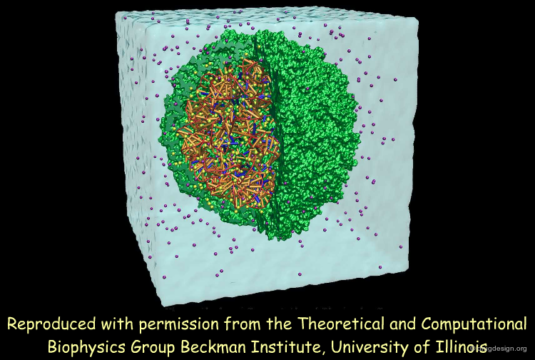
MD of the Complete Satellite Tobacco Mosaic Virus
In this seminal work, Klaus Schulten and colleagues used the NAMD package to perform all-atom MD simulations of a complete virus, the satellite tobacco mosaic virus. These simulations, with up to 1 million atoms for over 50 ns, were consistent with the stability of the whole virion and of the RNA core alone, suggesting at the same time that the capsid without RNA exhibits a pronounced instability. Large scale MD simulations of viruses may help unravel the mechanisms of the assembly and infection and their implications for treatment and prevention of viral infections.
articles
Molecular dynamics simulations of the complete satellite tobacco mosaic virus. Peter L. Freddolino, Anton S. Arkhipov, Steven B. Larson, Alexander McPherson, and Klaus Schulten Structure 14 2006
wikipedia
How Does RNA Moves Along DNA?
In order to understand how the RNA polymerase-II (Pol-II) enzyme moves along the DNA and how an unwound bubble of DNA is established and maintained in the transcription process, a model of the elongation complex in the pre-translocation state was constructed and studied by MD. The study revealed that several protein loops work concertedly to form and maintain the bubble structure. Also, a conformational change of one loop of the Pol-II enzyme works like a "heart valve", triggering the unidirectional movement of the RNA-polymerase-II along the DNA.

articles
Structure and dynamics of RNA polymerase II elongation complex Atsushi Suenaga, Noriaki Okimoto, Noriyuki Futatsugi, Yoshinori Hirano, Tetsu Narumi, Yousuke Ohno, Ryoko Yanai, Takatsugu Hirokawa, Toshikazu Ebisuzaki, Akihiko Konagay, Makoto Taiji Biochemical and Biophysical Research Communications 343 2006
wikipedia
Using MD for Conformational Sampling
The Sampling Approach in Optimization Problems
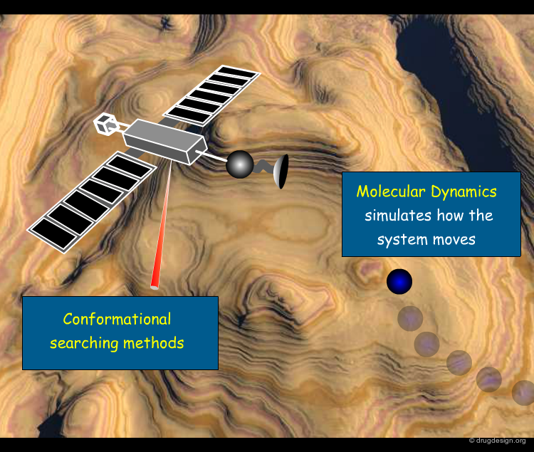
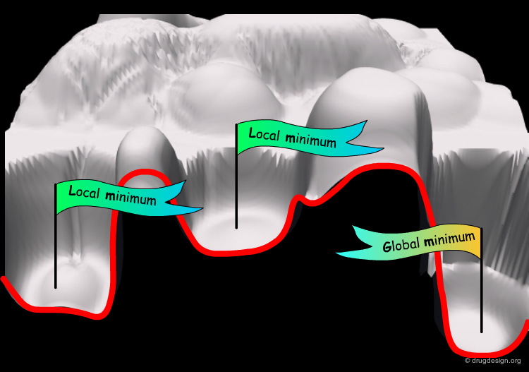
Finding the global minimum of a molecular system refers to an optimization problem for which there is no known algorithm that guarantees an optimal solution. MD can be used as an alternative approach to this problem by tracing the movement of a molecule in the conformational space. In conjunction with this issue, sampling approaches have emerged as a good alternative to the optimization problem as discussed in the following pages.

MD as a Tool for Sampling the Space
A molecular dynamics simulation calculates how a system moves on the potential surface. In this perspective, MD simulations can be used as a tool for sampling the space and tracing conformers all along the potential surface. When large macromolecules are involved, the dimensionality of the problem may become untenable. Different methods for sampling the conformational space of a system using MD dynamics as a tool are discussed here.

Sampling to Find the Global Minimum
Sampling consists of visiting possible configurations (conformations) of the system and can be performed using MD. In particular, MD can be used to sample preferred conformations of the system that correspond to local minima of the potential energy surface. Examples of applications for finding the global minimum and other low energy conformations are presented in the following pages.
wikipedia
Conformational Analysis of a Small Molecule
Organic molecules may have several rotatable bonds with several million conformations. The conformational analysis of a molecule aims at finding its low energy conformers. MD is a method of choice for sampling the conformational space of a molecule to find its preferred conformers.

Conformational Analysis of Biomolecules
The knowledge of the preferred conformations of a biomolecule is of utmost importance because these structures determine its biological properties and function.

Loop Conformation in Proteins
The prediction of the conformation of a loop in a protein is an issue that can be seen as a mini protein folding problem that also represents a typical example of the global minimization problem. The longer the loop, the higher the complexity of the problem.

How Do Ligands and Receptors Bind Together?
What are the orientation and geometries of a ligand and a receptor when they bind together? A ligand can interact with a protein in a number of different ways and accurate energy calculations are required to discriminate between them. This is another example of the global minimization problem, which is important in drug design.

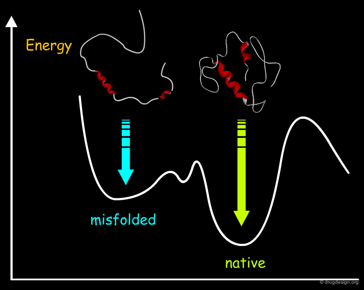
Protein Folding Problem
How does a protein adopt one unique specific native conformation and what is this conformation? This is the so-called protein-folding problem which represents another typical example of the global optimization problem encountered in computational biology. This issue has become of key interest to researchers because of the numerous protein sequences generated by the genome projects and by the discovery that the misfolding of proteins can lead to disease.
Systematic and Random Sampling
There are two main families of sampling approaches: the systematic and the random approaches. MD simulations are systematic, although not exhaustive. The Monte Carlo approach which will be presented later is a truly random approach.

wikipedia
Alternative Methods for Sampling
Monte Carlo, simulated annealing, diffusion equation and replica exchange methods are examples of random searches that can be used as an alternative to (or in conjunction with) molecular dynamics for sampling the conformational space.

Monte Carlo Random Search
Monte Carlo (MC) is a simulation technique of conformational sampling and optimization based on a computer algorithm that generates a series of random "moves" in order to identify energetically favorable conformations. The advantage of the MC method is its generality and a relatively weak dependence on the dimensionality of the system.

wikipedia
Monte Carlo Algorithm
The core of the Monte Carlo algorithm is a heuristic prescription for a plausible pattern of changes in the configurations assumed by the system. Such an elementary "move" depends on the type of the problem. For instance a rotation around a torsion angle or a combination of different ones may be determinant. A long series of random moves is generated with only some of them considered "good" moves.
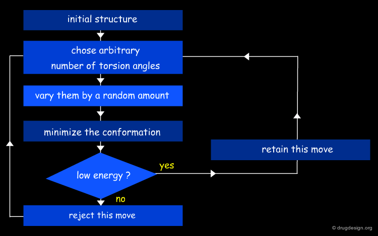
Metropolis Monte Carlo Approach
The Metropolis method is one type of a Monte Carlo simulation. The algorithm is based on statistical mechanics treatments combined with random moves. In the standard Metropolis MC a move is accepted unconditionally if the new configuration results in better (lower) potential energy. Otherwise it is accepted with a probability given by the Boltzmann factor (see below). The method is often employed because of its simplicity.

Simulated Annealing
The annealing process is a technique used in metallurgy where a metal is heated and then slowly cooled to obtain a crystalline structure with low internal energy. Molecular dynamics simulated annealing is a random-based sampling method that works by analogy with this process. It starts by an initial heating of the system and, in the second phase the temperature is gradually reduced. The process gives the system an opportunity to overcome energetic barriers, explore the entire potential surface and find the global minimum.
wikipedia
Diffusion Equation Methods
The diffusion equation method is based on smoothing the energy function and is an alternative to simulated annealing. Once the surface has been smoothed, the global minima can be rapidly found. The original rugged landscape can be smoothed out, for example by adding a Gaussian with a specific width at each point.

Replica Exchange MD Method
The "replica exchange MD" method (REMD) consists of running a number of simulations at different temperatures. Coordinates are exchanged at adjacent temperatures with some probability (following generalized Metropolis criteria) in order to prevent trapping in local minima. Because each replica can undergo cycles of heating and cooling, the potential surface is explored broadly.

articles
Replica-exchange molecular dynamics method for protein folding Yuji Sugita and Yuko Okamoto Chemical Physics Letter 314 1999
Replica exchange molecular dynamics simulations of amyloid peptide aggregation M. Cecchini, F. Rao, M. Seeber, and A. Caflisch Journal of Chemical Physics 121 (21) 2004
MD for the Calculation of Binding Energies
In Silico Drug Design
Computer experiments and simulations can be used to discover and design new molecules. Testing the properties of a molecule using computer modeling is faster and less expensive than synthesizing and characterizing it in a real experiment. Drug design by computer is now commonly used in the pharmaceutical industry. The calculation of free energies is among the most important applications of MD in drug design and this is discussed on the following pages.

articles
Combining docking and molecular dynamic simulations in drug design Alonso H, Bliznyuk AA, Gready JE Med Res Rev 26(5) 2006
Inhibitors of HIV-1 protease: a major success of structure-assisted drug design. Wlodawer A and Vondrasek J Annual Review of Biophysics and Biomolecular Structure 27 1998
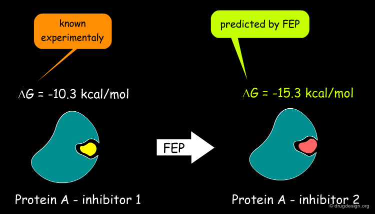
FEP Approach for Calculating Binding Energies
MD can be used to calculate relative affinities of ligand binding in conjunction with the so-called free energy perturbation (FEP) methods. It aims to predict the free energies of binding of new ligands from knowledge of the experimental binding energy of a known reference compound.
book
Reddy, M. Rami; Erion, Mark D. Free Energy Calculations in Rational Drug Design Springer - Verlag 2001
FEP Thermodynamic Cycle
Let us consider the thermodynamic cycle represented below. The free energy change between A and C is the same whether we go between them via B or D. We can write ΔG2 + ΔG3 = ΔG1 + ΔG4, which is equivalent to: ΔG3 - ΔG1 = ΔG4 - ΔG2. This equation gives us the difference between the two ligands' free energies of binding in terms of two other free energies that are easier to compute.
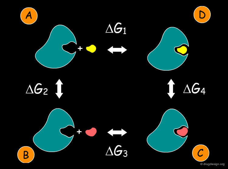
Exploiting the Thermodynamic Cycle
(ΔG3-ΔG1) gives the difference in binding energy between the two complexes. This quantity is of utmost importance because it enables us to compare the potency of the two ligands. Based on equation (1) this value is equal to (ΔG4-ΔG2). ΔG2 requires the calculation of the energies of the isolated ligands. ΔG4 is easy to compute, involving only the mutation of one ligand into the other. ΔG4 is calculated by MD as explained on the next page.

FEP: Computational Alchemy
The FEP method consists of the gradual change of the structure of the known ligand to that of the new one. For example imagine the progressive modification of benzene into methyl-cyclopentadiene. This is not possible experimentally but perfectly feasible computationally (a process sometimes called "computational alchemy"). The gradual change of the potential surface (U) of one molecule to the other can be achieved by the gradual change of Λ in equation (1) from the value Λ=0 (U=U1) to the value Λ=1 (U=U2).

Limitation of FEP Method
FEP has proven to give good results when the structural changes between the molecules to be compared are small. It is preferable to rely on the calculation of relative free energies rather than on absolute values, because systematic errors are cancelled out. The method can also apply to protein-protein interactions, for example in point-mutation studies.

FEP Study: Example 1
FEP calculations were used to estimate the contribution of each amino-acid of a small peptide MDM2 antagonist derived from the p53 transactivation domain. This revealed the importance of three amino-acids (Phe, Trp, Leu) and enabled the design of non-peptidic antagonists mimicking these residues.

articles
Discovery of potent antagonists of the interaction between human double minute 2 and tumor suppressor p53 Garcia-Echeverria C, Chene P, Blommers MJ and Furet P J. Med. Chem 43 2000
Computational Alanine Scanning To Probe Protein-Protein Interactions: A Novel Approach To Evaluate Binding Free Energies Massova I, Kollman PA. J. Am. Chem. Soc. 121 1999
Structure-Based Design of Spiro-oxindoles as Potent, Specific Small-Molecule Inhibitors of the MDM2-p53 Interaction Ke Ding, Yipin Lu, Zaneta Nikolovska-Coleska, Guoping Wang, Su Qiu, Sanjeev Shangary, Wei Gao, Dongguang Qin, Jeanne Stuckey, Krzysztof Krajewski, Peter P. Roller, and Shaomeng Wang J. Med. Chem. 49 2006
Discovery and Cocrystal Structure of Benzodiazepinedione HDM2 Antagonists That Activate p53 in Cells Bruce L. Grasberger, Tianbao Lu, Carsten Schubert, Daniel J. Parks, Theodore E. Carver, Holly K. Koblish, Maxwell D. Cummings et al. J. Med. Chem. 48 2005
Novel 1,4-benzodiazepine-2,5-diones as Hdm2 antagonists with improved cellular activity Leonard K, Marugan JJ, Raboisson P, Calvo R, Gushue JM, Koblish HK, Lattanze J, Zhao S, Cummings MD, Player MR, Maroney AC, Lu T. Bioorg Med Chem Lett 16(13) 2006
FEP Study: Example 2
Starting with a non-nucleoside HIV-1 reverse transcriptase inhibitor having an IC50 of 30 µM, Monte Carlo MD simulations with FEP enabled its rapid optimization to the 10 nM level.

articles
Computer-aided design of non-nucleoside inhibitors of HIV-1 reverse transcriptase William L. Jorgensen, Juliana Ruiz-Caro,Julian Tirado-Rives, Aravind Basavapathruni, Karen S. Andersonb and Andrew D. Hamilton Bioorganic and Medicinal Chemistry Letters 16 2006
MD Packages
Examples of Popular MD Packages
Programs for MD simulations started to appear in the late 1950s. The most popular packages are shown below and listed in the order of their first publication date. Important progress has been made because many of them continue to be actively maintained and enhanced. A brief outline of these programs is given on the following pages.

NAMD
NAMD is a parallel, object-oriented molecular dynamics code designed for high-performance simulation of large biomolecular systems. NAMD is file-compatible with AMBER, CHARMM, and X-PLOR and is distributed free of charge with source code.

wikipedia
VMD
VMD is a molecular visualization program for displaying, animating, and analyzing large biomolecular systems using 3-D graphics and built-in scripting.

wikipedia
TINKER
The TINKER molecular modeling software is a complete and general package for molecular mechanics and dynamics, with some special features for polypeptides. TINKER has the ability to use any of several common parameter sets, such as AMBER, CHARMM, MM2, MM3, OPLS-AA and OPLS-UA.

AMBER
AMBER is one of the most popular MD packages and force fields, developed by Peter Kollman and collaborators at Cornell (1995). AMBER offers a number of alternative force fields, in fact, various implicit solvent and electrostatic models, and quantum mechanical (QM) extensions, including semi-empirical methods to facilitate parameterization of novel compounds.

articles
The Amber biomolecular simulation programs. D.A. Case, T.E. Cheatham, III, T. Darden, H. Gohlke, R. Luo, K.M. Merz, Jr., A. Onufriev, C. Simmerling, B. Wang and R. Woods. J. Comput. Chem. 26 2005
Amber:assisted model building with energy refinement. a general program for modeling molecules and their interactions. P. K. Weiner and P. A. Kollman. J. Comput. Chem. 2 1981
wikipedia
CHARMM
CHARMM (Brooks et al., 1983) is another very popular general purpose molecular mechanics (MM) and MD simulation program. In addition to standard applications for energy minimization, molecular dynamics simulations, vibrational analysis and thermodynamic calculations, CHARMM can be used in conjunction with other QM/MM packages. The program contains a comprehensive analysis suite and it has been continuously developed in the laboratory of Martin Karplus and several groups of collaborators over the past 20 years.
"The CHARMM program is a general purpose molecular mechanics and molecular dynamics simulation program"

articles
CHARMM: a program for macromolecular energy, minimization, and dynamics calculations. Brooks BR, Bruccoleri RE, Olafson BD, States DJ, Swaminathan S and Karplus M Journal of Computational Chemistry 4 1983
wikipedia
GROMACS
GROMACS is a versatile package to perform molecular dynamics and simulate the Newtonian equations of motion for systems with hundreds to millions of particles.

wikipedia
MOIL
MOIL is a versatile public domain MD package, developed by the group of Ron Elber. Some unique features of MOIL include path integral approaches and various approximate sampling models, such as Locally Enhanced Sampling.
articles
MOIL: a program for simulation of macromolecules. Elber R, Roitberg A, Simmerling C, Goldstein R, Li H, Verkhivker G, Keasar C, Zhang J and Ulitsky A Computer Physics Communication 91 1994
book
Simmerling C, Elber R and Zhang J () The Proceeding of the Jerusalem Symposium on Theoretical Biochemistry. Kulwer Academic Publishers, Netherlands. 1995
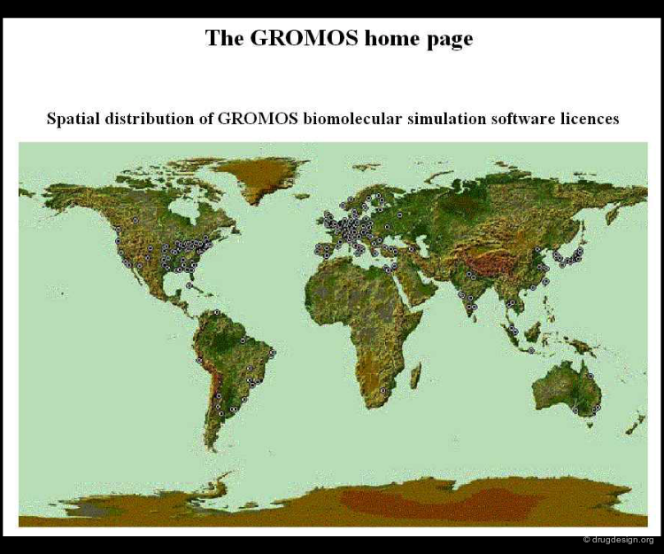
GROMOS
GROMOS is a general-purpose molecular dynamics computer simulation package for the study of biomolecular systems. Its purpose is threefold: (1) simulation of arbitrary molecules in solution or a crystalline state; (2) stochastic dynamics and (3) analysis of conformations obtained by experiment or by computer simulation. A force field is provided for proteins, nucleotides and sugars.
articles
Computer Simulation of Molecular Dynamics: Methodology, Applications and Perspectives in Chemistry W.F. van Gunsteren and H.J.C. Berendsen Angew. Chem. Int. Ed. Engl. 29 1990
On the interpretation of biochemical data by molecular dynamics computer simulation W.F. van Gunsteren and A.E. Mark Eur. J. Biochem. 204 1992
Fundamentals of drug design from a biophysical viewpoint W.F. van Gunsteren, P.M. King and A.E. Mark Quart. Rev. Biophysics 27 1994
Computer simulation of protein motion W.F. van Gunsteren, P.H. Huenenberger, A.E. Mark, P.E. Smith and I.G. Tironi Computer Phys. Communications 305-319 1995
wikipedia
Limitations and Perspectives
Limitations of MD
The crucial advantage of simulations is the ability to expand the horizon of the complexity that separates 'solvable' from 'unsolvable' issues. In this section, we consider some of the inherent limitations of empirical force fields and other limitations of Newton's equations of motion (EOM). In particular, the stability of the numerical integration of EOM, the problem of long range interactions and computational complexity (all contributing to the resulting time limitations in MD simulations) will be discussed.

Error Introduced by Empirical Potentials?
Standardized force fields are incorporated in the well established MD packages but are far from being invariant. The system remains under the influence of the user who introduces or removes constraints, energy contributions etc...; concomitantly this alters the "system" and its associated potential surface. There is enormous fuzziness in the use of approximate potential functions and this makes the quantification of the errors introduced in a simulation very difficult.

Trade Off Between Efficiency and Accuracy
Quantum (first principles) MD is computationally expensive; this triggered the development of effective alternatives in the form of empirical force fields. However, empirical force fields suffer from inherent limitations. Numerous approximations and problems with parameterization make the design of accurate (i.e. approximating closely the forces experienced by the "real" atoms), transferable (i.e. applicable to possibly many systems under different conditions), and computationally efficient force fields a challenging task.

Supramolecular Systems
Currently available force fields, such as AMBER or CHARMM, have been demonstrated to be sufficiently accurate for many applications of MD to simulations of proteins, membranes and nucleic acids. A whole domain of supramolecular chemistry was opened up by the seminal work of J.M. Lehn and others that has been abundantly studied with MD. However the coming era of long-time simulations for large and complex systems will pose new challenges in terms of stability and accuracy of MD and systematic techniques for improving the quality of the atomic force fields are highly desirable.

articles
Toward complex matter: supramolecular chemistry and self-organization. Lehn JM Proc Natl Acad Sci U S A. Apr 16;99(8) 2002
Supramolecular chemistry Lehn JM. Science Jun 18;260(5115) 1993
Toward self-organization and complex matter Lehn JM. Science Mar 29;295(5564) 2002
Supramolecular Co(II)-[2 x 2] Grids: Metamagnetic Behavior in a Single Molecule Waldmann O, Ruben M, Ziener U, Muller P, Lehn JM Inorg Chem. Aug 7;45(16) 2006
Lecon inaugurale, College de France, Paris Lehn, J.M. Interdisciplinary Science Rev. 10 1985
CHARMM: a program for macromolecular energy, minimization, and dynamics calculations. Brooks BR, Bruccoleri RE, Olafson BD, States DJ, Swaminathan S and Karplus M Journal of Computational Chemistry 4 1983
book
Lehn, J.M.
Weinheim: Wiley-VCH 1995
Long Range Forces as a Computational Bottleneck
Updating the positions and velocities in the stepwise numerical integration procedure requires recomputing the forces acting upon the atoms (which change their relative positions each time frame). The repeated summation over all pairs of atoms to compute interaction energies is time-consuming and constitutes a major bottleneck in MD simulations. Even when using smart methods, the overall complexity may be prohibitive for very large systems. Thus, the effective time scales accessible to MD simulations decrease significantly as the size of the system increases.
Time and Size Limitations
The time limitation is probably the most severe problem in MD simulations. Because of the presence of significant fast motions, the time step in numerical integration is typically limited to about 1-2 femtoseconds. Thus, folding a small protein (such as the villin headpiece in explicit solvent simulations) requires hundreds of billions of steps for a system consisting of thousands of atoms! To make the situation worse, multiple trajectories are required to derive relevant thermodynamical properties.

Alternative Techniques for Long Time Dynamics
The massively parallel MD approaches may not be sufficient to simulate long time dynamics of very large systems. This has stimulated the development of alternative techniques for long time dynamics such as implicit solvent models that greatly reduce the computational complexity of the problem.

From Impossible to Feasible
Attempts to study the dynamic behavior of a large system having more than 180.000 atoms (F1-ATP synthase in water) at the nanosecond level is summarized below. Progressively, and through a series of important efforts, the "impossible" task has proven to be doable.

articles
Nanoseconds molecular dynamics simulation of primary mechanical energy transfer steps in F1-ATP synthase R.A. Boeckmann and H. Grubmueller Nature Structural Biology 9 2002
Classical MD is not for Bond Breaking Mechanisms
The fixed covalent structure makes it impossible to use empirical potentials to directly model changes in chemical bonding that occur in the course of a chemical reaction. To study the reaction path of a chemical transformation such as the one illustrated below, it is necessary to do the simulation by calculating the energy with quantum mechanical methods.

Present and Future
Original MD simulations covered less than 10 ps in length for molecules of about 500 atoms. Recent developments show that greater simulation times can be reached (100 ns - 1 µs) and for much larger systems (100.000 - 1.000.000 atoms). Experts aim now to study more complex molecular and supramolecular systems to eventually arrive at the cellular level. Current attempts in the field provide a glimpse of the new frontiers and progress that will define the future of MD simulations.

articles
CHARMM: a program for macromolecular energy, minimization, and dynamics calculations. Brooks BR, Bruccoleri RE, Olafson BD, States DJ, Swaminathan S and Karplus M Journal of Computational Chemistry 4 1983
Simulations of protein folding and unfolding Brooks CL 3rd Current Opinion in Structural Biology 8 1998
Stability of alfa-helices. Chakrabar A and Baldwin RL Advances in Protein Chemistry 46 1995
A second generation force field for the simulation of proteins and nucleic acids. Cornell WD, Cieplak P, Bayly CI, Gould IR, Merz KM Jr, Fergusson DM, Spellmeyer DC, Fox T, Caldwell JW and Kollman PA Journal of American Chemical Society 117 1995
Pathways to a protein folding intermediate observed in a 1-microsecond simulation in aqueous solution. Duan Y and Kollman PA Science 282 1998
MOIL: a program for simulation of macromolecules. Elber R, Roitberg A, Simmerling C, Goldstein R, Li H, Verkhivker G, Keasar C, Zhang J and Ulitsky A Computer Physics Communication 91 1994
Flexible docking and design. Rosenfeld R, Vajda S and DeLisi C Annual Review of Biophysics and Biomolecular Structure 24 1995
Models and simulations of ion channels and related membrane proteins. Sansom MS Current Opinion in Structural Biology 8 1998
Biomolecular Simulation: The GROMOS96 Manual and User Guide. Zurich van Gunsteren WF, Billeter SR, Eising AA, Huenenberger PH, Krueger P, Mark AE, Scott WRP and Tironi IG Vdf Hochschulverlag
1996
Simulations of the molecular dynamics of nucleic acids. Auffinger P and Westhof E Current Opinion in Structural Biology 8 1998
Molecular dynamics simulations of biomolecules: longe-range electrostatic effects. Sagui C and Darden TA Annual Review of Biophysics and Biomolecular Structure 28 1999
book
Kuczera K Recent developments in theoretical studies of proteins World Scientific, Singapore 1996
Simmerling C, Elber R and Zhang J () The Proceeding of the Jerusalem Symposium on Theoretical Biochemistry. Kulwer Academic Publishers, Netherlands. 1995
Allen MP and Tildesley DJ Computer Simulation of Liquids. Oxford; Clarendon. 1987
Brooks CL 3rd, Karplus M and Pettitt BM A Theoretical Perspective of Dynamics, Structure and Thermodynamics. Wiley Interscience, New York. 1988
Protein Folding. Freeman and Company, New York 1992
Frenkel D and Smit B Understanding Molecular Simulation. From Algorithms to Applications. Academic Press, San Diego. 1996
Heile JM Molecular Dynamics Simulations: Elementary Methods. Wiley, New York. 1992
McCammon JA and Harvey SC Dynamics of Proteins and Nucleic Acids. Cambridge University Press, Cambridge 1987
Copyright © 2024 drugdesign.org